Priority Queues with Binary Heaps

Priority Queues with Binary Heaps in Swift. 2

Swimming Up the Tree.

In the last entry, we created a Priority Queue in Swift using an unordered array. In that case, when new items stream into the queue, they are added to the end regardless of their value. Then when the Priority Queue becomes too big, we remove the smallest item regardless of its position in the queue. That’s the unordered Priority Queue.
We could make a small variation of this and keep the Priority Queue ordered by adding each new item to its proper position in the queue right away. In this case, the queue never gets out of order. And when the queue is too big, we just delete the end item from the queue. That is called an Ordered Priority Queue.

Either the Ordered Priority Queue or the Unordered Priority Queue are good implementations if the queue is always going to be small.

But we can increase our efficiency by utilizing a Binary Heap. To understand this, consider a binary tree. The image below is a complete binary tree, which is defined as a tree that is balanced on all levels except for the bottom level, which may or may not be balanced.

In the image this tree with a height of 4 and 31 nodes. Each increase in the height occurs at a power of two. Thus if we had 32 nodes, the height of the tree would be 5.

Notice also that in our binary tree we are requiring each node to be bigger than its children. 95 is at the top. Its children, 70, and 80, are each smaller. And their children are also smaller.

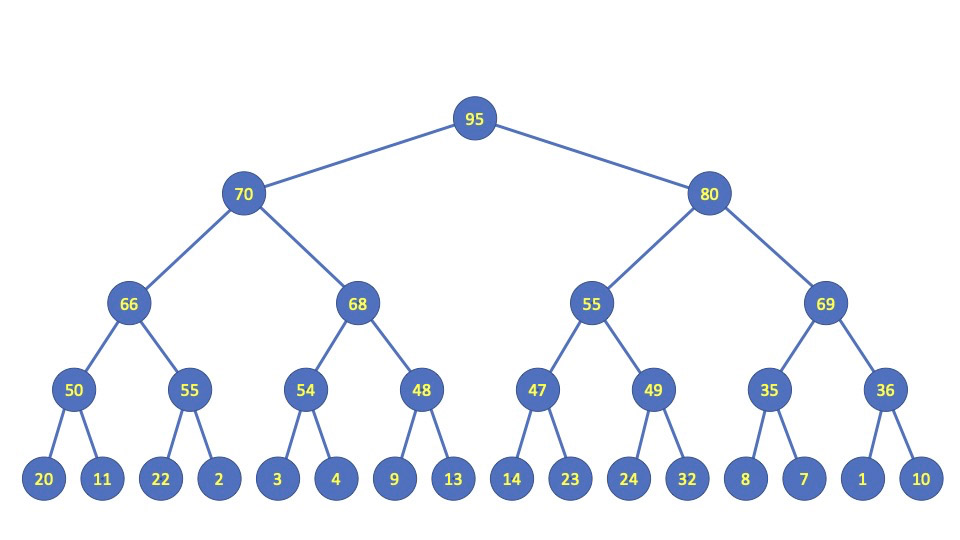
We will use the tree by placing our keys in nodes. In our example, that means each node will hold a movie receipt and its value.

We’ll get to that later. But for now, we’ll place arbitrary values in each node. These are our keys.

And again, we will ensure that the parent key is always greater or equal to each of its children.

We don’t have to represent this data as a tree. We can instead represent it as an array. In practice this is easier as we will see.

To represent the tree as an array, we add each level of the tree sequentially to the array, as in the next image:

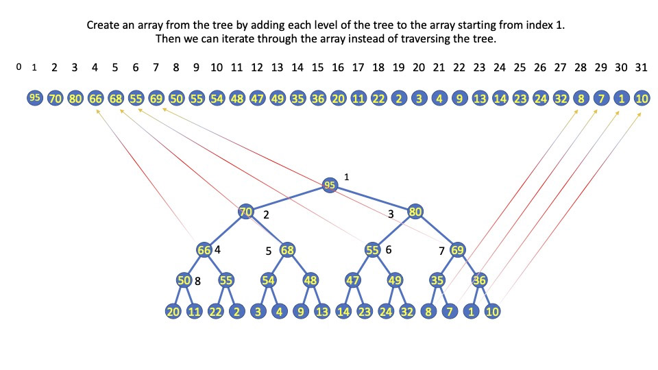
If the array is a, then a[1] is the largest value and is the root of the tree. In this case, the value is 95. We create the array from left to right using the level order of the tree, as indicated by the arrows.

Now for the magic math that we get by building the array from the tree:

Let’s call each index of the array i. If a node is at position i = 12, then its parent is always at position with an index of  i/2 = 6.

And its children are at index positions 2i and 2i + 1, or 24 and 25.

In the picture the value at i=12 is 47. The position in the array at index 12 has a value of 47. The position in the tree at index 12 — where we are traversing the tree across each level — has a value of 47.

Its parent is at i/2 = 6, and its value is 55. Its children are at positions 24 and 25.

These are the values 14 and 23.

Consider one more thing before wrapping up for today:  Consider how to resolve the problem when a node in the tree is bigger than a parent.

In that case, we will simply exchange the child with the parent. If the node that is now in the parent is still bigger than its parent, then we exchange again. This process of moving a node up the tree until all its children are smaller is called swimming up the tree.

We’ll code that in part III, and go further into how the Binary Tree helps us with the Priority Queue.