Introduction

In previous articles we learned what eigenvalues represent and how to calculate them. We showed what these concepts mean by analogy, including how the eigenvector might be considered the representative vector in a transformation: It’s the ribbon that flies straight out among all the other ribbons on the old oak tree. And we also learned how to calculate eigenvectors and eigenvalues.

Now we get to see the practical applications of eigenvalues to real neural network analysis. And by the end, we’ll be able to download our own layers from ChatGPT2, T5 and Bert and analyze them on our local computer. Yes these are the real professional-level layers.

Understanding the analysis and the results depends on understanding eigenvalues. We could skip to the end, download the python script and run it to graph the ChatGPT analysis right now without a real understanding. It will pop up a nice set of graphs.

Before we do that, lets take a high altitude look at what we’re talking about.

Spectral Analysis is X-ray Vision into Neural Networks.

Singular Value Decomposition — SVD — shows you all the most important parameters of your network layers.

Eigenanalysis is in some ways a simple version of SVD. It’s a subset of SVD. It only works under limited circumstances. But it’s very much related. Here we will stay focused on SVD.

SVD lets you compress the network based on the important directions; understand what the network learned by understanding what features were most important; debug training programs; and optimize fine tuning of your network.

Here we’ll learn about Spectral Analysis. This term encompasses both eigenanalysis and SVD. It’s one of the most exciting areas of machine learning, because this analysis tells you where the knowledge is inside that multibillion parameter monster!

When people say “spectral analysis of neural networks,” they mean, first of all, looking at the distribution of either eigenvalues or singular values or both.

When we look at eigenvalues, it’s called Eigenanalysis. And it is limited to looking at square matrices. In our previous papers we talked about what eigenvalues and eigenvectors are, and how you calculate them for small matrices. All of our calculations were limited to square vectors. And though we didn’t talk about that limitation at the time, it’s true: The matrices were square because that’s a requirement to find eigenvalues. We then went through methods to calculate them with a computer. And that’s the only practical method to calculate them with large matrices. The result of eigenanalysis is called an eigenvalue spectrum. And the word spectrum is really just a way to describe that we are looking at all the eigenvalues and their vectors. We are looking at the spectrum of things. We are looking at the range of eigenvalues.

Continuing from our earlier analogy to one eigenvalue being the straight ribbon, Eigenanalysis means identifying every direction where the transformation just stretches/compresses without twisting the ribbon. It means measuring each ribbon’s stretch factor. And it means understanding the complete transformation by looking at the ribbons that stay straightest (the largest eigenvalues) and also those which barely move (the smallest eigenvalues).

But most layers in a modern neural network are NOT square. And because of that, Eigenanalysis will not work. Instead we use a very similar technique called singular value decomposition — SVD.

When we look at singular values it’s called decomposition. And the spectrum we analyze is called the singular value spectrum. It’s nice to know that there is an exact mathematical relationship between singular values and eigenvalues. So if someone tells you that singular values are ‘like’ eigenvalues, you should know that the relationship is much tighter than ‘like.’ We will talk about it later. But we can be comfortable in thinking that if we understand eigenvalues, we are, in fact, much closer to understanding singular values.

Again, when people say “spectral analysis of neural networks,” they mean eigenanalysis or singular value decomposition. And they mean understanding which values are large and which are small. And they mean examining how the spectrum is structured in order to assess the network. For example: Is it uniform? Does it follow a power-law? Or does it have some other defining characteristics that we need to adjust before we release it to the world? We will get to all of that. But let’s dive right in by performing SVD on a small matrix. This example will help us learn the terms.

SVD by Hand Using the Smallest Matrix.

Singular value decomposition calucations by hand become very tedious even for a relatively small 3X3 matrix. But we want to be world class engineers, so we want to understand how to do it ourselves. Therefore, we’ll look at a very simple 2X2 matrix. It’s the simplest interesting case.

Along the way, we will find the three components of the SVD formula. These are U, s, and V.T. The formula is here:

Notice the order of the variables: U is sometimes called the ‘Left’ eigenvectors. V.T is sometimes called the ‘Right’ eigenvectors. And ‘s’ is an array of singular values arranged along the diagonal of a matrix.

Our starter example is this 2X2 matrix:

This is symmetric and full-rank. Here are the 5 steps to calculate it followed by a verification step 6.

Step 1. Compute W @ W.T — The ‘Gram’ Matrix.

This might be called ‘W times its transpose.’ It’s also called the ‘Gram’ matrix. Weighty name. We’ll go into the term later.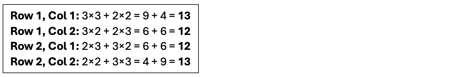

So W @ W.T — the Gram matrix — is this: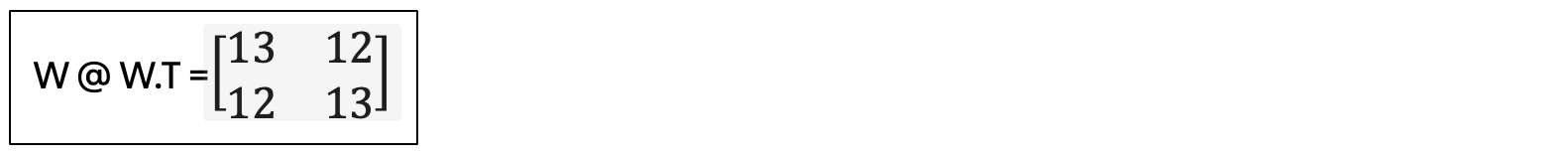

Step 2. Find Eigenvalues of W @ W.T

We already knew that eigenvalues would be important. We need to solve for the eigenvalues of W.

To do this, we recognize that the determinate of the Gram matrix minus the eigenvalue times the identity matrix must be zero.

But we just need to solve for lambda.

Thus we solve: det(W @ W.T — λI) = 0

Expand the determinant: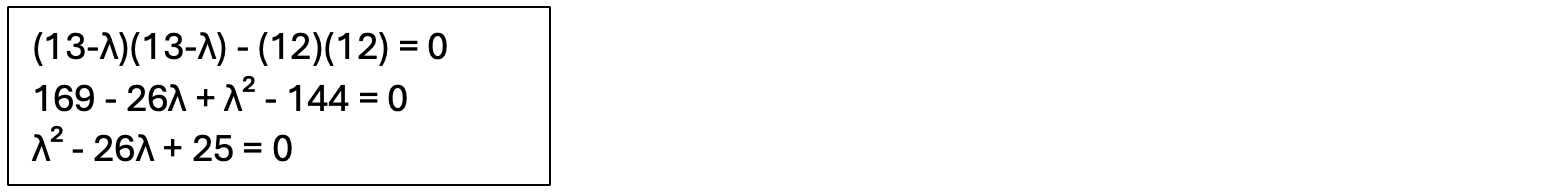

Use the quadratic formula: λ = (-b ± √(b²-4ac)) / 2a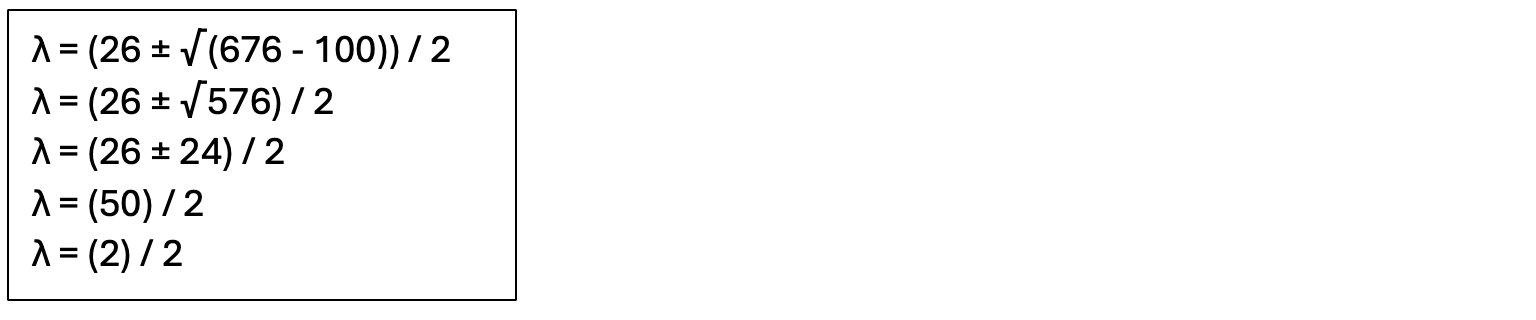

And we find the eigenvalues:

λ₁ = 50/2 = 25
λ₂ = 2/2 = 1

Step 3. Compute the Singular Values

Singular values are the square roots of eigenvalues. Earlier we mentioned that there was a direct mathematical relationship between eigenvalues and singular values. This is that relationship. We had two eigenvalues. So we calculate two singular values and put them in an array called ‘s.’

s₁ = √25 = 5
s₂ = √1 = 1

So: s = [5, 1].

That’s the middle of our SVD formula. But nobody calls it the middle. They just call U the left and V.T the right.

Step 4. Find Eigenvectors for U, the Left Singular Vectors

We have two eigenvalues. We will solve for the eigenvectors as we have previously.

The equation we use to find the eigenvectors from the eigenvalues is this:

And solving for the first eigenvalue, λ₁ = 25:

Solve: (W @ W.T — 25I) v = 0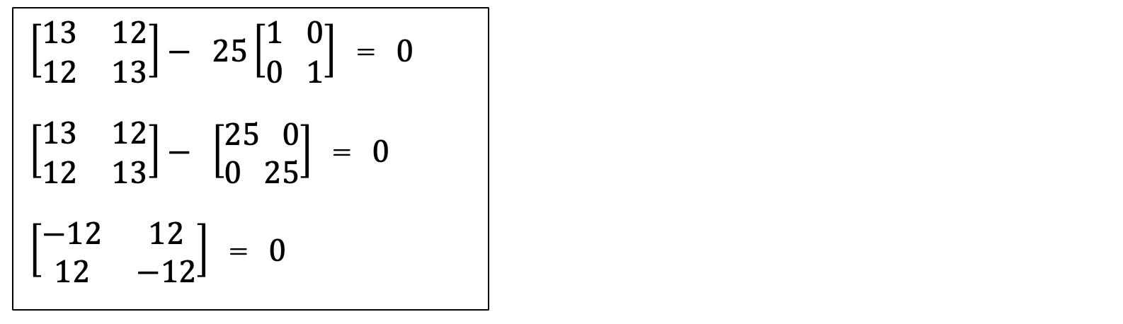

Equation: -12v₁ + 12v₂ = 0.

Solving for the equation, we see that v₁ = v₂.

So we can arbitrarily assign v1 = 1, and therefore v2 = 1. The vector with these two values is [1, 1].

And therefore the vector with all its values normalized is the square root of the sum of the squares:

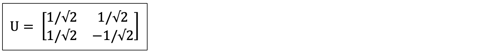
Normalized: v₁ = [1/√2, 1/√2] ≈ [0.707, 0.707]

For the second eigenvalue:

For λ2 = 1:

Solve: (W @ W.T — 1I) v = 0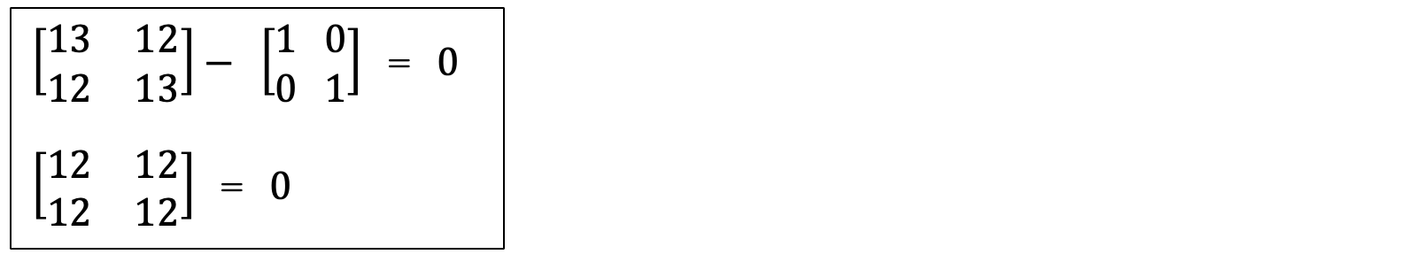

Equation: 12v₁ + 12v₂ = 0.

Solving for the equation, we see that v₁ = -v₂.

So we can arbitrarily assign v1 = 1, and therefore v2 = -1. The vector with these two values is [1, -1].

And therefore the vector with all its values normalized is the square root of the sum of the squares:

Normalized: v₁ = [1/√2, -1/√2] ≈ [0.707, -0.707]

And with these two vectors, we have the vectors in U, the left singular vectors:

At this point we have the left singular vectors and the middle singular values. We need one more thing:

Step 5. Find Eigenvectors for V, the Right Singular Vectors

For a symmetric matrix like ours, W.T @ W = W @ W, so V = U! Therefore we don’t have another real calculation to do. We simply recognize that V = U: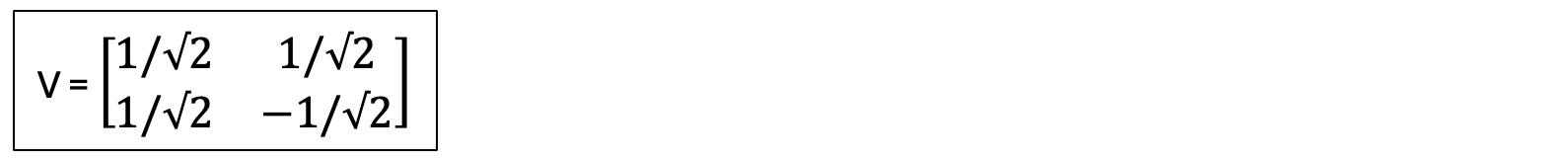

And of course in this case, V.T = V. So now we can assemble all three parts of the SVD equation.

Final SVD Result: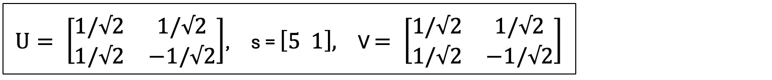

Now let’s verify our numbers.

Step 6. Verify by Reconstruction

To verify, we return to the original SVD equation and multiply it out. Here’s that original equation again:

And if we fill in the values we obtained above, here is what we will start with before we multiply it out:

First, let us multiply U — the left singular vectors — times the singular values in the middle: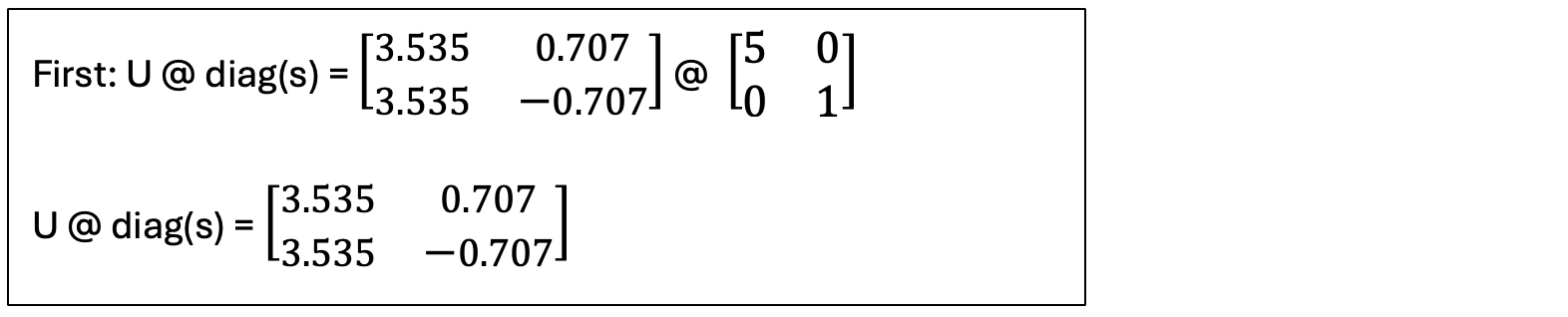

Second, let us multiply the result of that by V.T:

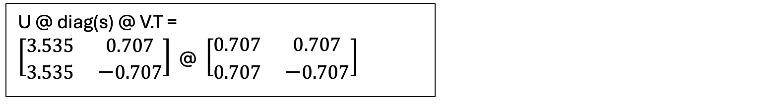
Here are the individual products

Row 1, Col 1: 3.535×0.707 + 0.707×0.707 = 2.5 + 0.5 = 3 ✓
Row 1, Col 2: 3.535×0.707 + 0.707×(-0.707) = 2.5–0.5 = 2 ✓
Row 2, Col 1: 3.535×0.707 + (-0.707)×0.707 = 2.5–0.5 = 2 ✓
Row 2, Col 2: 3.535×0.707 + (-0.707)×(-0.707) = 2.5 + 0.5 = 3 ✓

We got back to our original matrix W:

That’s it. Here are the key points to remember:

First: We have been looking at the Gram matrix, or the matrix multiplied by its transpose.

Second: Singular values, s, are the square roots of eigenvalues of the Gram matrix.

Third: The eigenvectors of the Gram matrix are the ‘left singular vectors’ in the variable ‘U.’

Fourth: For symmetric matrices, U = V.

Fifth: We use the ‘SVD’ formula ‘W = U @ diag(s) @ V.T’ to reconstruct the original matrix from U, s, and V.

We did this exercise to get more practive in eigenvalues, to understand the relationship between eigenvalues and singular values, and to give ourselves a better understanding of what is going on when we calculate singular values of larger matrices and can’t reasonably do the math by hand.

What we missed in this small example was why SVD works on non-square matrices and Eigenanalysis only works on square matrices.

The Why of SVD Variable Names.

From above, you saw the SVD formula, which we expressed as this:

But is usually expressed like this:

Just to be clear, the ‘@’ sign represents a matrix transformation. And in the latest expression of the SVD formula, we are using the symbol ‘ Σ ‘ to represent an array of all the singular values, placed on the diagonal of a matrix.

Matrix operations usually proceed right to left.

Since V.T is on the right side, it is called the ‘right singular vectors.’

U is on the left side so this is called the ‘left singular vectors.’

Here’s a critical take-home message:

There is a deeper concept to make clear. We are doing SVD analysis and not eigenanalysis in part because the layers of our network are not square. But also because the shape of our input matrix is seldom the same as the shape our our output.

Despite that fact, we want to learn how which vectors in our input space most strongly affect the vectors in our ourput space.

That was the critical message. We just passed it, in case you weren’t paying full attention.

Imagine a coffee barista. In this example, they are using four ingredients (4-dimensional input): Beans, cream, sugar and cinnamon. And they are concerned with three characteristics of the coffee (3-dimensional output): sweetness, aroma and bitterness.

You can’t ask: “Which ingredient stays the same after mixing?” That question doesn’t make sense. Sugar becomes sweetness; coffee adds to bitterness; cream reduces the bitterness; cinnamon changes the aroma, but so does the bean and the cream.

But the mixture transforms the coffee and its ingredients into a different thing.

SVD helps us keep track of this. It asks two different questions:

Question 1 (Measured as the Input Space matrix that we call ‘V’):

"Which combinations of ingredients have the strongest effect on the output?"

The results might be described as directions:
• Direction 1: Mostly sugar + cream → creates strong sweetness
• Direction 2: Mostly beans + cream → creates richness
• Direction 3: Mostly cinamon → creates aroma
• Direction 4: Random mix → barely affects anything
These directions are the right singular vectors (V). 
These are the important directions in ingredient space – which 
we also know as input space.

Question 2 (Measured as the Output Space matrix that we call ‘U’):

"Which flavor combinations do we actually get out?"

These results might also be described as directions:
• Direction 1: Mostly sweetness (from the sugar + cream combo)
• Direction 2: Mostly richness (from beans + cream combo)
• Direction 3: Mostly aroma (from cinamon)
These are the left singular vectors (U) - These are the important directions in flavor space – which we also know as the output space.

Why are there “Two Spaces”? The Input space (4D) is where the ingredients live; the output space (3D) is where the flavors live. These are different spaces — you can’t compare them directly! But SVD lets us look at them.

SVD finds V, the best ingredient combinations (in 4D ingredient space); U, what flavors they produce (in 3D flavor space), and s, how strong each connection is between the ingredients and the flavors.

Now to bring it home, consider why eigenanalysis doesn’t work: Eigenanalysis would ask: ‘Which ingredient vector stays an ingredient vector?’ But that’s impossible, because when you mix the ingredients they become flavors. SVD asks instead, ‘What’s the best way to organize the ingredients to produce the flavors I want?’

Later we will analyze the ChatGPT layer, with 768 inputs and 2304 outputs. And we’ll see which of the 768 inputs matter most to the 2304 outputs.

The Key Insight from this section is that for SVD, ‘Both spaces’ means the space where the data starts (the inputs), and the space where the data ends up (the outputs). When they’re different dimensions, you need different directions for each!

We are not ready to analyze layers of ChatGPT just yet. We have a few more steps to go before we can tackle that big goal.

We will next go through a progression of examples to begin to understand the utility of SVD when we later use it to analyze full fledged transformer layers. We will start with the diagonal matrix.

SVD of a Diagonal Matrix.

This is the first teaching example. It’s a special case. Note that when we start with a diagonal matrix, the result is already obvious. We’ll see that in a moment, after we work our way to the result.

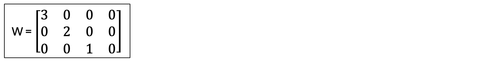
The shape is 3X4, and it maps 4 dimensional to 3 dimensional space.

Step 1. Compute W @ W.T, also known as the Gram Matrix.

This might be called ‘W times its transpose.’

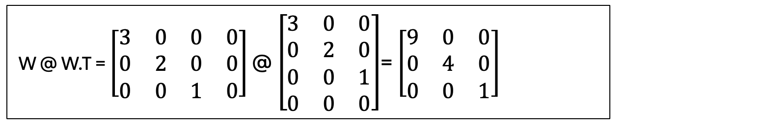
The result is already diagonal! This tells us the eigenvectors are the standard basis.

That’s because for any diagonal matrix D:

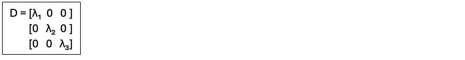
The eigenvectors are always the standard basis vectors:

• e₁ = [1, 0, 0]ᵀ with eigenvalue λ₁
• e₂ = [0, 1, 0]ᵀ with eigenvalue λ₂
• e₃ = [0, 0, 1]ᵀ with eigenvalue λ₃

Step 2. Find the Eigenvalues

Next, the characteristic equation is this: det(W @ W.T — λI) = 0. So we will write it out for our values as this:

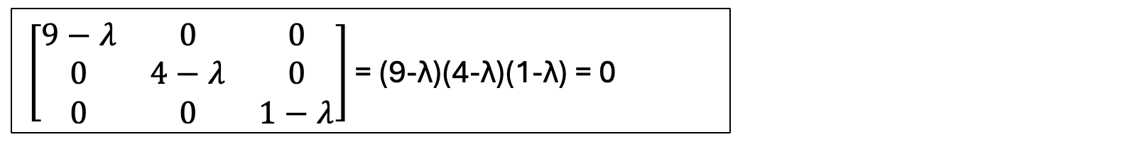
And from this we find the Eigenvalues: λ₁ = 9, λ₂ = 4, λ₃ = 1

Step 3. Expand the Determinant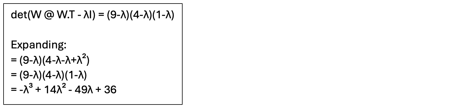

Then set the equation to zero:

And find the roots: λ = 9, 4, 1.

This verifies that we hve the correct eigenvalues.

Step 4. Compute Singular Values

Remember that the singular values are the root of the eigenvalues: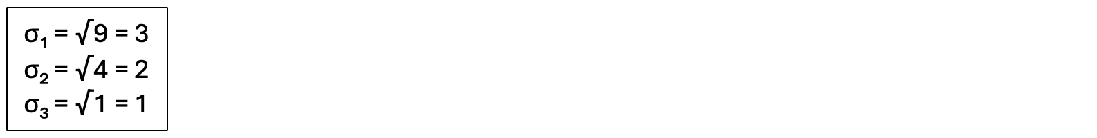

Now you can see that the singular values are exactly the diagonal entries of W! We did the work to earn this result.

Step 5. Find U (The Left Singular Vectors)

The left singular vectors are the eigenvectors of W @ W.T:

Again we are calculating the eigenvectors from the eigenvalues.

For λ = 9: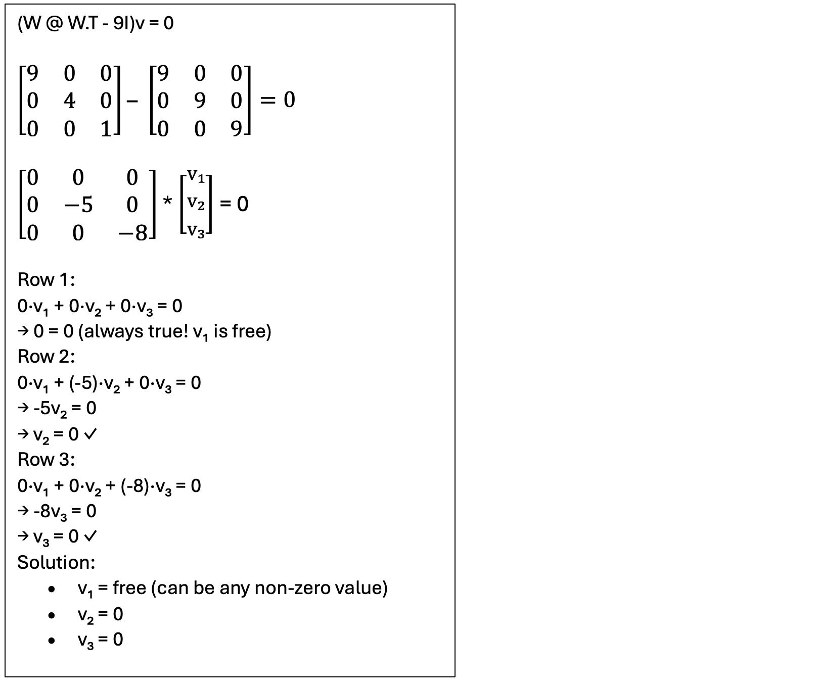

Since v₁ = free, we can set it to 1. And the solution for λ = 9, and our first eigenvector, is:

Finding the solutions for the other two singular values means solving these two equations:

And the solutions are:

For λ = 4:

For λ = 1:

And the final solution for U — all the left singular vectors — is this: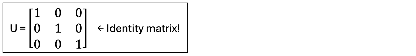

U is the identity matrix!

Step 6. Find V (The Right Singular Vectors)

To find V, we need to compute W.T @ W, which will be a 4X4 vector: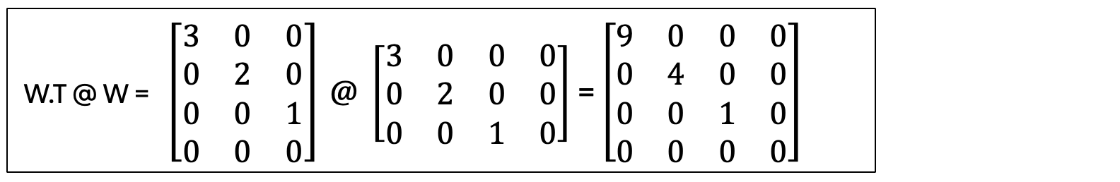

And here the eigenvalues are 9, 4, 1, 0 (where we have one zero because we lost rank).

And using the basis vectors as the eigenvectors again, we can calculate V: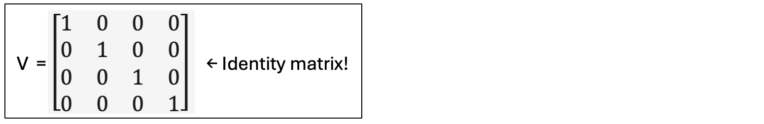

Step 7. Final SVD Decomposition

Like before, we represent the SVD using the more formal equation:

And here is what we calculated: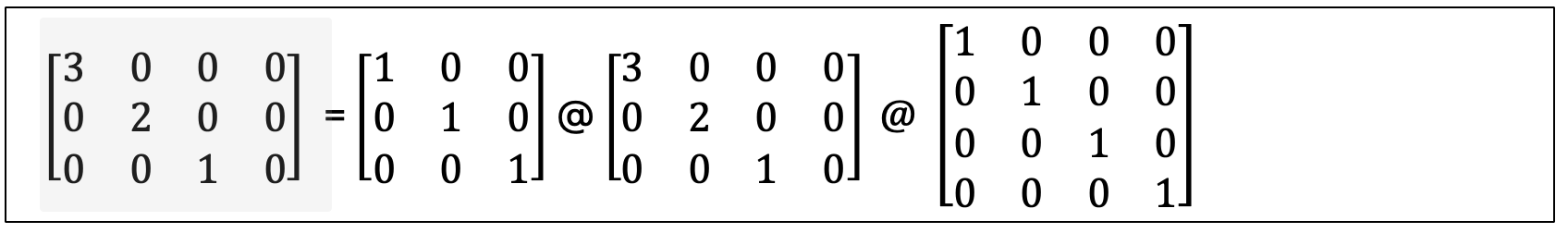

What did we learn from this example? There is a general principle. A matrix is diagonal if and only if it’s already expressed in its eigenvector basis. That’s what makes this example so perfect — we’re already in the “natural” coordinate system! In this special case, we wanted to show some special features. They don’t always apply. Remember the following:

• The coordinate axes are already aligned with the stretching directions.

• Singular values appear directly because they’re the diagonal entries.

• U and V are identity matrices — no change of basis required.

But in this case we also wanted to repeat some more generic features of SVD calculations. This is how our example connects to the general algorithm:

• W @ W.T always gives you U and σ² (the square of σ — the singular value — is the eigenvalue). This is true even when W is not a diagonal matrix.

• W.T @ W always gives you V and σ². Also true when W is not a diagonal matrix.

So here’s a ‘secret’ worth keeping close. It will help you in future analyses: The Gram matrix is what we’ve been using all along. U and V are each different Gram matrices. The Gram matrix G of vectors v₁, v₂, …, vₙ is the matrix of all pairwise inner products.

That’s important.

The Gram matrix is the matrix of all pairwise inner products.

Because of this, we can think of the Gram matrix as a holistic geometric fingerprint of the matrix. That’s why it’s important in SVD. In fact since both U and V are Gram matrices, we might say that the concept of a Gram matrix is really fundamental to SVD.

There are some nuances to this argument. But as beginners, we can think of the Gram matrix as a means to generate a simplifed representation of a complex matrix. That’s really what we are doing here after all.

Now that you know that, let’s add a second, deeper secret:

When the Gram matrix is diagonal, the vectors are orthogonal. SVD’s job is to find a rotation that makes the Gram matrix diagonal.

Why is this important? We can think of orthogonal vectors as those vectors that are most meaningful and most independent of other information. This is the information in a layer of a neural network that we want to preserve the most. Fields such as ‘linux kernel’ and ‘18th century court customs’ are very independent of each other. Their mathematical representation in a network would have a high likelihood of being represented on orthogonal vectors. So if we want our network to focus more on linux and less on knights, we will be able to tune the network representation of one without changing the other. That’s because their vectors are orthogonal.

We just went through an example where the vectors started out as orthogonal. SVD’s job is to find a rotation that makes the Gram matrix diagonal in general cases! So that we can find all the biggest clusters of orthogonal vectors. And with that, find the most meaningful parts of our network. (Without even knowing what knowledge is hidden there!)

In summary, this example shows the “target” of SVD. It doesn’t show any of the special types of interpretations we can get out of SVD. That is, it doesn’t really show how we can use SVD to analyze matrices or layers of a network.

That starts next.

SVD of a Rank Deficient Matrix.

This is the second teaching example. It’s another special case. Here we start with a rank-deficient matrix.

Rank deficient matrices are those that have rows that are duplicates, or are multiples of other rows, or are sums of other rows. These rows are not linearly independent.

And we can evaluate this with singular values. Consider the following matrix where the second row is twice the first and the third row is three times the first:

This example is instructive because, as mentioned, all rows are multiples of the first.

Also: the singular values are:

And two singular values are essentially zero. This shows a rank-1 structure. And this is ‘rank collapse’ in neural networks.

The important message is this: When a matrix as small as a 3X4 matrix only has a rank 1, SVD reveals this immediately with near-zero singular values. It tells us we have a ‘weak’ network with poor use of our weights.

SVD of a Low Rank Matrix.

Consider the next example: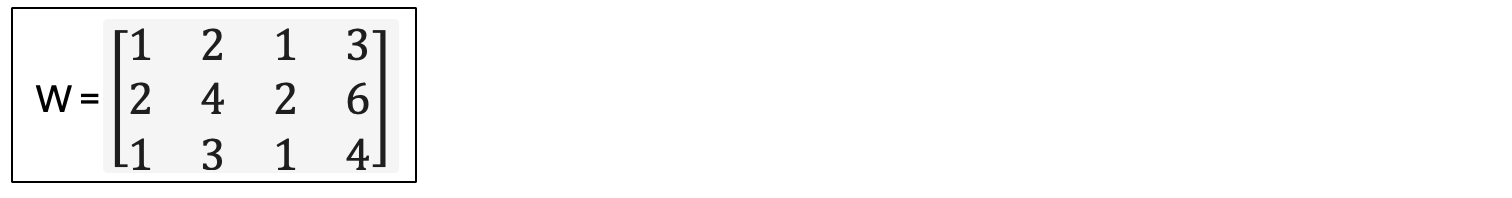

This is a low rank matrix, but the rank is not immediately obvious by looking. In fact it’s a rank 2 matrix. And the calculation of the singular values will show that the third singular value is ~0.

This is similar to what is seen in neural networks: A hidden low-rank structure. It’s something easily revealed by SVD. And in this case you can verify it by observing that row 3 ~= (row 1 + row 2)/ 2.

Here the important message is this: SVD can reveal hidden redundancy that is not obvious from inspection.

SVD of a Full Rank Matrix with Power-Law Decay

This is the third teaching example and this the most neural-network-like situation. There are singular values for every row.

But the singular values decay.

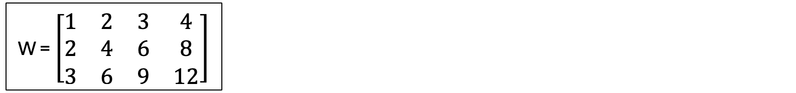
Take the following matrix: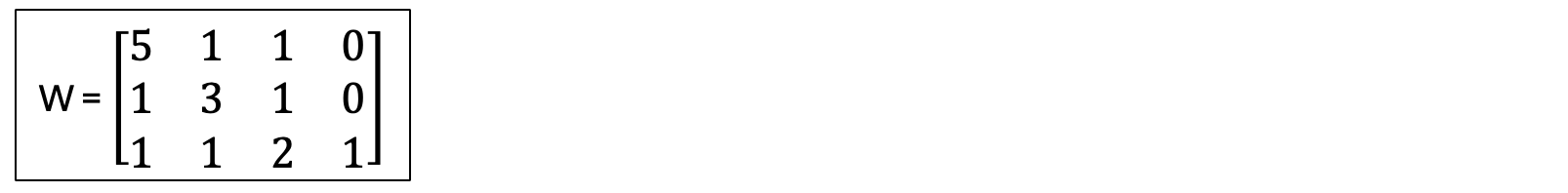

With a full rank matrix, there is a nonzero singular value for every row. But the singular values decay. Perhaps they look like this:

In this case the first singular value dominates. In some cases you may see large dominance of a few singular values. Like this:

This means most information flows in a few directions and many directions carry little information.

On the other hand, in some networks a higher power-law decay is expected. In computer vision early layers show strong power-law decay because natural images have strong correlations where neighboring pixels on the screen are often similar.

In general, if we can capture 90% of the signal with 10% of the dimensions, that’s considered efficient learning. In the code example with the ChatGPT2 layer, this is the ‘cumsum’ and in the console you will see it as the ‘Rank-10 approximation.’ Look through the examples after running that code and we will find variations in the Rank-10 with the different layers. But they all hover near 10%.

Now let’s consider computer-calculated SVD values. The first example is small. After that we consider actual models like ChatGPT2 (and two others).

SVD of a Small Matrix.

Consider the following python code, which we can easily run in VS Code:

import numpy as np

import numpy as np

# A tiny 3x4 matrix with integer values
W = np.array([
    [1, 2, 3, 4],
    [5, 6, 7, 8],
    [9, 10, 11, 12]
])

print("Original matrix W:")
print(W)
print(f"Shape: {W.shape}")

# Perform SVD
U, s, Vh = np.linalg.svd(W, full_matrices=False)

print("\n=== SVD Results ===")
print(f"\nLeft singular vectors U: {U.shape}")
print(U)

print(f"\nSingular values s: {s.shape}")
print(s)

print(f"\nRight singular vectors Vh: {Vh.shape}")
print(Vh)

# Reconstruct to verify
W_reconstructed = U @ np.diag(s) @ Vh
print("\nReconstructed matrix (should match original):")
print(W_reconstructed)

print("\nDifference (should be ~0):")
print(np.max(np.abs(W - W_reconstructed)))

The output we should expect in the console is below:

Original matrix W:
[[ 1  2  3  4]
 [ 5  6  7  8]
 [ 9 10 11 12]]
Shape: (3, 4)

=== SVD Results ===

Left singular vectors U: (3, 3)
[[ 0.20673589  0.88915331  0.40824829]
 [ 0.51828874  0.25438183 -0.81649658]
 [ 0.82984158 -0.38038964  0.40824829]]

Singular values s: (3,)
[2.54368356e+01 1.72261225e+00 2.64839734e-16]

Right singular vectors Vh: (3, 4)
[[ 0.40361757  0.46474413  0.52587069  0.58699725]
 [-0.73286619 -0.28984978  0.15316664  0.59618305]
 [ 0.26153473 -0.70741401  0.63022384 -0.18434456]]

Reconstructed matrix (should match original):
[[ 1.  2.  3.  4.]
 [ 5.  6.  7.  8.]
 [ 9. 10. 11. 12.]]

Difference (should be ~0):
1.7763568394002505e-15

First we are seeing the matrix and its shape. W is a 3 X 4 matrix.

Then we make a numpy call to perform the singular value decomposition for us.

Here is the call itself:

It’s a simply numpy call from the linear algebra package called ‘svd.’ It returns a tuple with three values: U, s, and Vh.

The result then shows us the three left singular vectors, the three singular values and the three right singular vectors.

And likewise the variable ‘V’ is also just a standard matrix name that we often see for SVD. But here it’s followed by an ‘h.’ The ‘h’ stands for ‘Hermitian transpose.’ But for our purposes, with real matrices (as opposed to complex matrices) it will always be the same as a regular transpose. And transposing a matrix means writing the rows as columns or vice versa. So in python, the transpose of V would be written ‘V.T’ and therefore ‘Vh = V.T’

This was a brief introduction to the computation of U, s and Vh. Now that we know what the call looks like, we can apply it to large network layers.

SVD of a Real ChatGPT Transformer Layer

Here we’ll use singular value decomposition to look at the properties of a real neural network transformer layer from ChatGPT-2. And if you download the code from this github gist, you’ll see how to look at the properties of ANY public layer.

First, let’s clarify typical layer shapes in GPT-style models.

Typical Layer Shapes in GPT Model Attention Layers.

These layers consist of Q, K, V projections: 768 → 768 (GPT-2 small), 1024 → 1024 (GPT-2 medium), 1280 → 1280 (GPT-2 large).

When we talk about “one layer” in a transformer like GPT-2, we mean one transformer block, which contains:

1. One Multi-Head Attention (one sublayer with 3 matrices)
• Q (Query) matrix: 768 → 768
• K (Key) matrix: 768 → 768
• V (Value) matrix: 768 → 768
These are three separate weight matrices that work together 
as part of the attention mechanism. They're all part of the 
same "attention sublayer."

And

2. One Feed-Forward Network (one sublayer with 2 matrices)
• First projection: 768 → 3072 (expansion)
• Second projection: 3072 → 768 (compression)

So “One Layer” = 5 Weight Matrices Total. Here’s another illustration of the layer we want to exmine: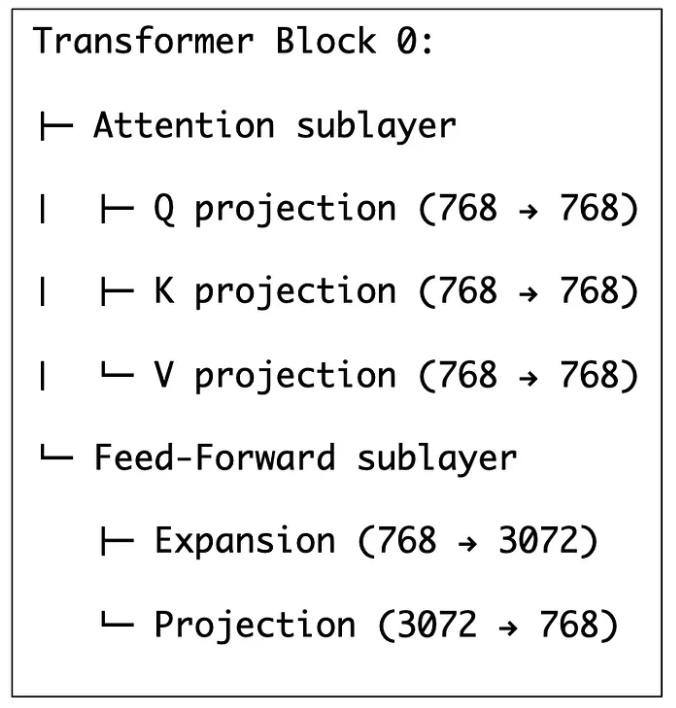

In the python code example, look for this:

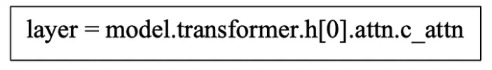
This is where we load the transformer layer.

Look also for commented-out areas that you can use to load layers from other models. The code is already there, you simply need to choose the model you want to examine.

In the case of ChatGPT2, we’re actually getting all three (Q, K, V) combined into one big matrix: 768 → 2304 (because 768 × 3 = 2304). And because this is not a square matrix, as we know well by now, it is not suitable for eigenanalysis.

Run the code:

import torch
import numpy as np
from transformers import GPT2LMHeadModel
import matplotlib.pyplot as plt

# ===== MODEL SELECTION =====

# Option 1: GPT-2 (current)
model = GPT2LMHeadModel.from_pretrained('gpt2')
layer = model.transformer.h[0].attn.c_attn  # Combined Q,K,V projection
model_name = "GPT-2 (117M params)"

# Option 2: BERT - Encoder-only architecture (110M params)
# from transformers import BertModel
# model = BertModel.from_pretrained('bert-base-uncased')
# layer = model.encoder.layer[0].attention.self.query  # Just the Query projection
# model_name = "BERT-base (110M params)"

# Option 3: T5 - Encoder-decoder architecture (60M params - small version)
# from transformers import T5Model
# model = T5Model.from_pretrained('t5-small')
# layer = model.encoder.block[0].layer[0].SelfAttention.q  # Query projection in encoder
# model_name = "T5-small (60M params)"

# ===========================
# First, let's explore the model structure
print("Model structure:")
for name, module in model.named_modules():
    if isinstance(module, torch.nn.Linear):
        print(f"{name}: {module.weight.shape}")

# Now let's grab a specific layer - the first attention layer's query projection
W = layer.weight.data.cpu().numpy()

print(f"\nWeight matrix shape: {W.shape}")

# Spectral Analysis 1: Singular Value Decomposition
U, s, Vh = np.linalg.svd(W, full_matrices=False)

cumsum = np.cumsum(s**2) / np.sum(s**2)

print(f"\nSpectral Properties:")

# Calculate some useful metrics
effective_rank = np.sum(s)**2 / np.sum(s**2)  # Participation ratio
condition_number = s[0] / s[-1]

print(f"\nSpectral Properties:")
print(f"Effective rank: {effective_rank:.2f} / {len(s)}")
print(f"Condition number: {condition_number:.2e}")
print(f"Rank-10 approximation captures {cumsum[9]*100:.1f}% of variance")
plt.figure(figsize=(12, 4))

# Plot singular values
plt.subplot(1, 3, 1)
plt.plot(s)
plt.yscale('log')
plt.xlabel('Index')
plt.ylabel('Singular Value')
plt.title('Singular Value Spectrum')
plt.grid(True)

# Plot cumulative variance explained
plt.subplot(1, 3, 2)
plt.plot(cumsum)
plt.xlabel('Number of Components')
plt.ylabel('Cumulative Variance Explained')
plt.title('Effective Rank')
plt.grid(True)

# Spectral Analysis 2: Eigenvalues of W @ W.T (Gram matrix)
gram = W @ W.T
eigenvalues, eigenvectors = np.linalg.eigh(gram)
eigenvalues = np.sort(eigenvalues)[::-1]  # Sort descending

plt.subplot(1, 3, 3)
plt.plot(eigenvalues)
plt.yscale('log')
plt.xlabel('Index')
plt.ylabel('Eigenvalue')
plt.title('Eigenvalues of W @ W.T')
plt.grid(True)

plt.tight_layout()
plt.show()

input("Press Enter to exit...")  # keeps the process alive until you press Enter

Here’s what the output metrics tells us about this GPT-2 attention layer:

Weight matrix shape: (768, 2304)
This projects 768-dimensional embeddings to 2304 dimensions (3×768 for Query, Key, and Value matrices concatenated together).

Effective rank: 542.72 / 768
The matrix is using about 71% of its theoretical maximum rank — it’s not full-rank, meaning there’s some redundancy, but it’s using most of its representational capacity (not highly compressed).

Condition number: 4.55e+01
The largest singular value is 45× bigger than the smallest — this shows moderate “stretching” where some input directions get amplified much more than others, but it’s not extreme (the matrix is reasonably well-conditioned, not ill-conditioned).

Rank-10 approximation captures 12.9% of variance
The information is very distributed across many dimensions — we’d need to keep far more than 10 singular values to capture most of the transformation’s behavior (the matrix is definitely not low-rank, unlike what you might see in overparameterized or post-training compressed networks).

Overall takeaway: This is a healthy, information-rich weight matrix that spreads its representational power across hundreds of dimensions rather than concentrating it in just a few dominant directions.

Notice the plot of the data:

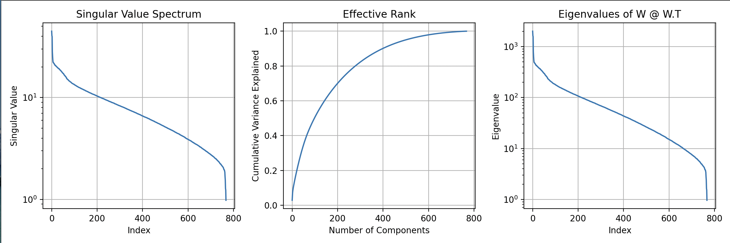
The graphs show us details:

Singular Value Spectrum

This graph shows the singular values in descending order — the smooth, gradual decay (no sharp “elbow”) means the transformation spreads information across many dimensions rather than compressing into just a few dominant directions. This indicates the layer is learning a rich, distributed representation, not a simple low-rank approximation.

Effective Rank

The cumulative variance curve shows you need ~400–500 components to capture 90%+ of the behavior — this curve confirms the matrix is high effective rank and not easily compressible. If this were a low-rank matrix (like after aggressive pruning), you’d see it shoot up to 100% much faster.

Eigenvalues of W @ W.T

These are the squared singular values (σ²) from the Gram matrix — they show the same smooth decay pattern but on a squared scale. The relationship is: eigenvalues = (singular values)², so the largest eigenvalue (~1⁰³) corresponds to the largest singular value (~30–35). This confirms the row-space geometry has the same distributed structure.

Conclusion:

We’ve gone through a lot! Isn’t ‘Spectral Analysis’ a neat term?

We have a great intuitive understanding of SVD analysis, and we’ve used that analysis on several examples to drive it home. And we used it computationally to examine a real public layer and output information about the quality of that layer.

Not to mention that you now know how to download public network layers into python code!

Coming back to the ribbon analogy: If your transformation takes 768 ribbons and outputs 3072 ribbons, there’s no single set of “straight ribbons.” Instead, SVD finds: 768 input directions (right singular vectors) and 3072 output directions (left singular vectors). And the singular values tell you how each input direction maps to output strength.

This is incredibly powerful math and a part of every AI engineer’s toolkit.

From here we have more analytical techniques to learn. And more math. That’s coming in future weekly articles.

Not only that, but there are several techniques for applying SVD to matrix analysis that we did not cover in this article. But even with this beginning, we can examine nearly any publicly available model in great detail.