

Implement The Recurrent Neural Network

The Elman RNN Implementation in Python
The Elman RNN Training Loop
Introduction
Variations in Network Structure and
Input.
Introduction
Elman’s publication ‘Finding Structure in Time’ (Cognitive Science, 1990) was an influencial demonstration of recurrent neural networks. That paper was reviewed in a separate publication by this author. Recurrent neural networks were important in the development of predictive text – a feature all of us see when texting from our phones every day. And they still play important roles in many neural networks and AI models today. Understanding how they work is fundamental to understanding the later development of gated neural networks, long short-term memory networks and even transformers.
In my view the best way to understand how they work is to create a functioning implementation. In this paper we walk through the implementation. We will use input similar to the input in two different experiments from Elman’s paper: In his first experiment, he used a stream of bits and trains the network to calculate the XOR representation of the bits. We will do the same. We will also repeat Elman’s second experiment, where he uses a stream of letters to train the network to recognize patterns in the letter sequences.
The complete code is available at my github repo here. We will describe it in overview first, then we will walk through each function.
At the end I suggest several variations that you can try to help you understand how well the network functions. It is possible to learn how many training epochs are needed to achieve Elman’s results. And it is possible to create networks with more or fewer hidden units and examine how that changes the training rate.
The Elman RNN Training Loop Introduction
The ‘training loop’ is a fundamental concept in machine learning.
In the most general sense, a training loop is called a loop because the network is fed input with the desired qualities. This is the forward step of training. And at the end of this forward step the network actual output value is compared to the known expected value. The difference between the actual output and the expected output is the loss. This loss value is used to correct the weights of the network in a back propagation step. Thus there is a forward step and a backward step – and this is the loop. The loop is executed multiple times.
In our implementation, we print out the magnitude of the loss during training. You’ll be able to see the loss decrease as training continues. You’ll gain an understanding of how changes in the loss reflect actual learning in the network.
We also print out the actual values and the expected values. This will help you understand where the network output is incorrect and why.
In the Elman paper, the string of bits used to train the XOR function is fed as input 600 times. In modern parlance, Elman subjected his network to 600 epochs of training. The input sequence that Elman used was 3000 bits. The python code for the first experiment will default to 600 epochs with a sequence of 3000 bits, just like Elman.
But since you have the code, you can modify any of these values. I’ll walk you through that.
Training Loop Code Overview
Here’s the complete training process overview.
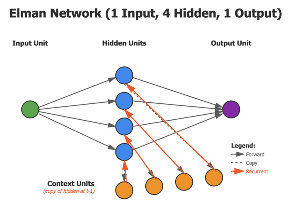
First, we will initialize the network. We will create a network with 4 hidden units, to match the network we describe in the Elman review paper, as seen in the figure below:
1. When we initialize the code for the XOR test, we will set the number of hidden units to 4. We use the same number for the context units. This happens in the __init__() function.
2. Next we go through the training loop! Find the code "for epoch in range(num_epochs):" Each time through the loop we call a ‘train_step’ where we go through both the forward and a backward training steps. Note that in this version, and in Elman’s version, we make a forward training step and then immediately make a measure of the loss and do the back propagation step. There are other versions of the RNN network that do multiple forward steps before doing any training. We won’t consider that version here.
That’s it. After these two steps, we present the data. We ‘ll go through that code. But these two steps are all you need for an overview. Now let’s start diving into the details.
Recreate the Network
1. From the main function, we can execute the XOR task or the cv (consonant-vowel) task or both. Here we will begin the XOR task. This is where we initialize the network by calling ElmanNetwork(). After that we will generate the input sequence.
def xor_task():
    """Test the XOR task"""
    print("=" * 70)
    print("XOR Task Test")
    print("=" * 70)

    # Create network for XOR (1 input, 4 hidden, 1 output)
    network = ElmanNetwork(n_input=1, n_hidden=4, n_output=1, learning_rate=0.1)

    # Generate XOR sequence
    sequence = generate_xor_sequence(3000, seed=42)
    print(f"First 15 bits: {sequence[:15]}")
    print()

    # Train network
    print("Training...")
    losses = network.train_sequence(sequence, num_epochs=600, verbose=True)
    print()

    # Test predictions
    test_sequence = sequence[:20]
    network.reset_context() #Reset context to zeros
    predictions = network.predict_sequence(test_sequence)

    print("Actual Output vs Expected Output:")
    print("Time | Input | Actual Out | Rounded Out | Expected | Match")
    print("-" * 60)

    correct = 0
    for i in range(len(predictions)):
        input_val = test_sequence[i]
        expect = test_sequence[i + 1]
        actual = predictions[i][0, 0]
        actual_rounded = 1 if actual > 0.5 else 0
        match = "✓" if expect == actual_rounded else "✗"

        if expect == actual_rounded:
            correct += 1

        print(f" {i:2d}  |   {input_val}   |   {actual:.4f}   |      {actual_rounded}      |     {expect}    |  {match}")


    accuracy = (correct / len(predictions)) * 100
    print("-" * 60)
    print(f"Accuracy: {correct}/{len(predictions)} = {accuracy:.1f}%")
    print()

    # Test predictions of third bit only.
    # Uncomment the following to see accuracy at only the XOR output positions.
    # print("Actual vs Expected Only At XOR Positions:")
    # print("Time | Input | Actual Out 3 | Rounded Out | Expected | Match")
    # print("-" * 60)

    # correct = 0
    # for i in range(1, len(predictions), 3):
    #     input_val = test_sequence[i]
    #     expect = test_sequence[i + 1]
    #     actual = predictions[i][0, 0]
    #     actual_rounded = 1 if actual > 0.5 else 0
    #     match = "✓" if expect == actual_rounded else "✗"

    #     if expect == actual_rounded:
    #         correct += 1

    #     print(f" {i:2d}  |   {input_val}   |   {actual:.4f}   |      {actual_rounded}      |     {expect}    |  {match}")

    # accuracy = (correct / (len(predictions) // 3)) * 100
    # print("-" * 60)
    # print(f"Accuracy3: {correct}/{round(len(predictions)/3)} = {accuracy:.0f}%")
    # print()

    # Error rate at each position.
    # I want something that looks at errors at each of the three positions separately.
    # I want the root mean square error at each position.
    # Uncomment the following to see error rates by position in group of 3.

    # position_errors = [0, 0, 0]
    # position_counts = [0, 0, 0]
    # for i in range(len(predictions)):
    #     input_val = test_sequence[i]
    #     expect = test_sequence[i + 1]
    #     actual = predictions[i][0, 0]
    #     actual_rounded = 1 if actual > 0.5 else 0

    #     pos = i % 3
    #     position_counts[pos] += 1
    #     if expect != actual_rounded:
    #         position_errors[pos] += 1
    # print("Error Rate by Position in Group of 3:")
    # print("Position | Errors | Total | Error Rate")
    # print("-" * 40)
    # for pos in range(3):
    #     errors = position_errors[pos]
    #     total = position_counts[pos]
    #     error_rate = (errors / total) * 100
    #     print(f"   {pos}     |  {errors:3d}  |  {total:3d} |   {error_rate:.2f}%")
    # print()

    return network, losses
2. Here we initialize the class. This function is where we set the number of hidden units and context units – the base architecture of the network. Here we also set the learning rate, the initial weights and biases. Note that the weights are initialized with random numbers. Also note that the context is initialized with zeros. Since the context represents the memory of the hidden values from the previous input, and there was not input yet, initializing them to zero seems to make sense. But you could argue that point.
    def __init__(self, n_input, n_hidden, n_output, learning_rate=0.1):
        """
        Initialize the Elman network
        Args:
            n_input: Number of input units
            n_hidden: Number of hidden units
            n_output: Number of output units
            learning_rate: Learning rate for gradient descent (default: 0.1)
        """

        self.n_input = n_input
        self.n_hidden = n_hidden
        self.n_output = n_output
        self.learning_rate = learning_rate

        # Initialize weights with small random values
        # W_ih: Input → Hidden (n_hidden x n_input)
        self.W_ih = np.random.randn(n_hidden, n_input) * 0.1

        # W_hh: Context → Hidden (n_hidden x n_hidden matrix)
        self.W_hh = np.random.randn(n_hidden, n_hidden) * 0.1

        # W_ho: Hidden → Output (n_output x n_hidden)
        self.W_ho = np.random.randn(n_output, n_hidden) * 0.1

        # b_h: Hidden biases (n_hidden x 1)
        self.b_h = np.zeros((n_hidden, 1))

        # b_o: Output bias (n_output x 1)
        self.b_o = np.zeros((n_output, 1))

        # Context units (initialized to zeros)
        self.context = np.zeros((n_hidden, 1))
3. Back in the xor_task(), you can see that after we initialize the network, we then jump to generate_xor_sequence() and generate the sequence used to train the network. As mentioned, the sequence is 3000 bits long by default. It’s is critical to understand the structure: It is a repeating pattern of three bits. The first bit is randomly chosen. The second bit is randomly chosen. The third bit is the XOR calculation of the first two bits. Then the pattern repeats. You can see this in the ‘for _ in range(num_groups):’ loop, where the three bits are calculated in a group, and then added to the growing sequence. The bottom line is that position matters. Only the third position is non-random.
def generate_xor_sequence(length=100, seed=None):
    """
    Generate XOR sequence in Elman's format: groups of (bit1, bit2, bit1 XOR bit2)

    Args:
        length: Total length of sequence (will be rounded down to nearest multiple of 3)
        seed: Random seed for reproducibility

    Returns:
        sequence: List of bits (0s and 1s) in groups of 3
    """
    if seed is not None:
        np.random.seed(seed)

    sequence = []
    num_groups = length // 3

    for _ in range(num_groups):
        bit1 = np.random.randint(0, 2)
        bit2 = np.random.randint(0, 2)
        xor_result = bit1 ^ bit2

        sequence.extend([bit1, bit2, xor_result])

    return sequence
4. Again going back to the xor_task(), you can see that after we generate the input sequence, we start the training with train_sequence(). The function train_sequence is the main workhorse for the class. It trains the recurrent neural network with a number of forward passes equal to the num_epocs, which we default to 600. Note that we are training for 600 epochs, but we use the same sequence each time. We are training the network to learn the patter of 1s and 0s that are needed to recognize the XOR pattern, which is 1 if the two previous digits are different, and 0 if the two previous digits are the same.
    def train_sequence(self, sequence, num_epochs=600, verbose=True):
        """
        Train on a complete sequence for multiple epochs
        Args:
            sequence: List of input values/vectors
            num_epochs: Number of times to iterate through sequence
            verbose: Whether to print progress
        Returns:
            losses: List of average loss per epoch
        """
        losses = []
        for epoch in range(num_epochs):
            # Reset context at start of sequence
            self.reset_context()
            total_loss = 0
            # Train on sequence
            for t in range(len(sequence) - 1):
                x = sequence[t]
                target = sequence[t + 1]
                output, error = self.train_step(x, target)
                # Accumulate error
                total_loss += error
            # Calculate average loss
            avg_loss = total_loss / (len(sequence) - 1)
            losses.append(avg_loss)
            # Print progress
            if verbose and (epoch + 1) % 10 == 0:
                print(f"Epoch {epoch + 1}/{num_epochs}, Loss: {avg_loss:.6f}")

        return losses
5. Previously, in train_sequence(), we loop through the 600 epochs, and for each epic we loop through the 1000 bits of the sequence. For each bit in the sequence, we call train_step(), which calls both the foward() and backward() passes to train the network.
    def train_step(self, x, target):
        """
        Complete training step: forward + backward + update context
        Args:
            x: Input value or vector
            target: Target output value or vector
        Returns:
            output: Predicted output
            error: Prediction error (MSE)
        """
        # Forward pass
        output, hidden = self.forward(x)

        # Backward pass
        error = self.backward(x, hidden, output, target)

        # Update context for next time step
        self.update_context(hidden)

        return output, error
6. The ‘forward’ function is where we process the input. It is the first function called in the ‘train_step’ function. Note that we calculate the hidden_input as the combination of the input and the context (along with the bias term). The actual value of the hidden units is the sigmoid of the hidden_input. After calculating the hidden layer, we calculate the output_input, which is the dot product of the weights and the hidden layer (along with the bias). Then the actual output is a sigmoid of the output_input.
    def forward(self, x):
        """
        Forward pass: compute hidden state and output for one time step
        Args:
            x: Input vector (n_input x 1) or scalar (for 1D input)
        Returns:
            output: Predicted output (n_output x 1)
            hidden: Hidden state (n_hidden x 1)
        """
        # Convert input to column vector if needed
        if np.isscalar(x):
            x_vec = np.array([[x]])
        elif x.ndim == 1:
            x_vec = x.reshape(-1, 1)
        else:
            x_vec = x

        # Compute hidden layer input
        # hidden_input = W_ih * x + W_hh * context + b_h
        hidden_input = np.dot(self.W_ih, x_vec) + np.dot(self.W_hh, self.context) + self.b_h

        # Apply sigmoid activation
        hidden = self.sigmoid(hidden_input)

        # Compute output layer input
        # output_input = W_ho * hidden + b_o
        output_input = np.dot(self.W_ho, hidden) + self.b_o

        # Apply sigmoid activation
        output = self.sigmoid(output_input)

        return output, hidden
7. Here we show two vital utility functions. If you are unfamiliar with the sigmoid function then refer to discussions about them I have written elsewhere. On the other hand, don’t dismiss these as ‘merely’ utility functions. These two functions are used everywhere in machine learning. They are vital.
     def sigmoid(self, x):
        """Sigmoid activation function"""
        x_clipped = np.clip(x, -500, 500)
        return 1 / (1 + np.exp(-x_clipped))

    def sigmoid_derivative(self, y):
        """Derivative of sigmoid function"""
        return y * (1 - y)
8. In the ‘backward’ function, we find the error – the distance that the output is from the expected result – and use the magnitude of that error to adjust all the weights in the network. In our case, we run the backward function once after each run of the forward function.
    def backward(self, x, hidden, output, target):
        """
        Backward pass: compute gradients and update weights

        Args:
            x: Input that was used (n_input x 1) or scalar
            hidden: Hidden state from forward pass (n_hidden x 1)
            output: Output from forward pass (n_output x 1)
            target: Target/desired output (n_output x 1) or scalar

        Returns:
            error: Mean squared error
        """
        # Convert scalars to proper shapes
        if np.isscalar(x):
            x_vec = np.array([[x]])
        elif x.ndim == 1:
            x_vec = x.reshape(-1, 1)
        else:
            x_vec = x

        if np.isscalar(target):
            target_vec = np.array([[target]])
        elif target.ndim == 1:
            target_vec = target.reshape(-1, 1)
        else:
            target_vec = target

        # 1. Compute output layer error
        error = output - target_vec
        delta_o = error * self.sigmoid_derivative(output)
        # 2. Compute hidden layer gradients
        delta_h = np.dot(self.W_ho.T, delta_o) * self.sigmoid_derivative(hidden)
        # 3. Update W_ho: Hidden → Output
        self.W_ho -= self.learning_rate * np.dot(delta_o, hidden.T)
        # 4. Update b_o: Output bias
        self.b_o -= self.learning_rate * delta_o
        # 5. Update W_ih: Input → Hidden
        self.W_ih -= self.learning_rate * np.dot(delta_h, x_vec.T)
        # 6. Update W_hh: Context → Hidden (recurrent)
        self.W_hh -= self.learning_rate * np.dot(delta_h, self.context.T)
        # 7. Update b_h: Hidden biases
        self.b_h -= self.learning_rate * delta_h
        # Return mean squared error
        return np.mean(error ** 2)
9. Back in the train_step() function, we have one more thing to do: Update the context. In the update_context function we set the ‘memory’ of the RNN. We simply copy the values of the hidden layer into the context layer. This is where the word ‘recurrence’ becomes relevant. That’s because the previous setting of the hidden layer becomes the memory and its use ‘recurs’ the next time a forward training event happens.
    def update_context(self, hidden):
        """Update context units with current hidden state"""
        self.context = hidden.copy()
10. After we update the context for the 6,000,000th
time, we are done with all the train_step calls. Every time we called the backward() function, we returned an error, which is a representation of the distance between the network output and the target. Also known as the ‘loss.’ The error is returned to train_step(), and from there it is returned to train_sequence() and appended to the array of loss values. You can see that this function has been storing the ‘loss’ value from every train_step call. At this stage, we can analyze our loss values and examine how well our network predicted the next values in the sequence. Our code flow exits train_sequence() and gets back to xor_task().
The function predict_sequence is called from xor_task() after training is complete. In this function, we put the newly trained network to work. We put in a sequence of ones and zeros (by default we will test with 20 values from the original sequence) and we ask the neural net to predict the next digit. The prediction is a probability and is put in the ‘predictions’ array and returned.
You’ll likely find that from the 20 tested values, the frequency of getting the XOR value correct is about 100%. In the first 20 values there are 6 XOR calculations. You can un-comment code in the xor_task() function to see the error by position. The errors in the other two (non-XOR positions) are much higher.
    def predict_sequence(self, sequence):
        """
        Use the trained network to predict next value for each position in sequence.

        Args:
            sequence: List of values/vectors

        Returns:
            predictions: List of predicted values/vectors
        """
        # Reset context
        self.reset_context() #Reset context to zeros

        predictions = []

        # Make predictions
        for t in range(len(sequence) - 1):
            x = sequence[t]
            output, hidden = self.forward(x)

            predictions.append(output)

            # Update context for next step
            self.update_context(hidden)
        return predictions
12. The main() function creates the network, generates the XOR sequence used in training, tests the network and generates a graph. You can input the type of test you wish to run as an input variable, using ‘xor’, ‘cv’, or ‘both’. We haven’t discussed the ‘cv’ task yet. We will do that next. For a complete discussion of both of these see my review of the Elman work in the companion paper.
def main(task='both'):
    """
    Run Elman network tasks

    Args:
        task: Which task(s) to run - 'XOR', 'CV', or 'both' (default)
    """
    task = task.upper()

    if task not in ['XOR', 'CV', 'BOTH']:
        print(f"Invalid task '{task}'. Must be 'XOR', 'CV', or 'both'")
        return

    xor_network = None
    xor_losses = None
    cv_network = None
    cv_losses = None
    bit_errors = None

    # Run XOR task if requested
    if task in ['XOR', 'BOTH']:
        xor_network, xor_losses = xor_task()

        if task == 'BOTH':
            print("\n" + "=" * 70 + "\n")

    # Run CV task if requested
    if task in ['CV', 'BOTH']:
        cv_network, cv_losses, bit_errors = cv_task()

    # Plot results if matplotlib available
    try:
        import matplotlib.pyplot as plt
        import os

        # Create outputs directory if it doesn't exist
        # Try /mnt/user-data/outputs first (for Claude), fall back to local ./outputs
        output_dir = '/mnt/user-data/outputs' if os.path.exists('/mnt/user-data') else './outputs'
        os.makedirs(output_dir, exist_ok=True)

        if task == 'BOTH':
            # Plot both tasks
            fig, axes = plt.subplots(2, 2, figsize=(14, 10))

            # XOR training loss
            axes[0, 0].plot(xor_losses)
            axes[0, 0].set_xlabel('Epoch')
            axes[0, 0].set_ylabel('Loss')
            axes[0, 0].set_title('XOR Task: Training Loss')
            axes[0, 0].grid(True, alpha=0.3)

            # CV training loss
            axes[0, 1].plot(cv_losses)
            axes[0, 1].set_xlabel('Epoch')
            axes[0, 1].set_ylabel('Loss')
            axes[0, 1].set_title('CV Task: Training Loss')
            axes[0, 1].grid(True, alpha=0.3)

            # CV bit errors (like Figure 5 from Elman)
            bit_names = ['Consonant', 'Vowel', 'Interrupted', 'High', 'Back', 'Voiced']

            # Plot bit 0 (Consonant)
            axes[1, 0].plot(bit_errors[0, :30], 'o-', markersize=4)
            axes[1, 0].set_xlabel('Time Step')
            axes[1, 0].set_ylabel('Squared Error')
            axes[1, 0].set_title(f'Bit 1: {bit_names[0]}')
            axes[1, 0].grid(True, alpha=0.3)

            # Plot bit 3 (High)
            axes[1, 1].plot(bit_errors[3, :30], 'o-', markersize=4)
            axes[1, 1].set_xlabel('Time Step')
            axes[1, 1].set_ylabel('Squared Error')
            axes[1, 1].set_title(f'Bit 4: {bit_names[3]}')
            axes[1, 1].grid(True, alpha=0.3)

            plt.tight_layout()

            save_path = os.path.join(output_dir, 'elman_tasks_comparison.png')
            plt.savefig(save_path, dpi=150, bbox_inches='tight')
            print(f"\nPlots saved to: {save_path}")

        elif task == 'XOR':
            # Plot only XOR
            plt.figure(figsize=(10, 5))
            plt.plot(xor_losses)
            plt.xlabel('Epoch')
            plt.ylabel('Loss')
            plt.title('XOR Task: Training Loss')
            plt.grid(True, alpha=0.3)

            timestamp = datetime.now().strftime('%Y%m%d_%H%M%S')
            filename = f'elman_xor_training_{timestamp}.png'
            save_path = os.path.join(output_dir, filename)
            plt.savefig(save_path, dpi=150, bbox_inches='tight')
            print(f"\nPlot saved to: {save_path}")

        elif task == 'CV':
            # Plot only CV
            fig, axes = plt.subplots(1, 3, figsize=(15, 4))

            # CV training loss
            axes[0].plot(cv_losses)
            axes[0].set_xlabel('Epoch')
            axes[0].set_ylabel('Loss')
            axes[0].set_title('CV Task: Training Loss')
            axes[0].grid(True, alpha=0.3)

            # CV bit errors (like Figure 5 from Elman)
            bit_names = ['Consonant', 'Vowel', 'Interrupted', 'High', 'Back', 'Voiced']

            # Plot bit 0 (Consonant)
            axes[1].plot(bit_errors[0, :30], 'o-', markersize=4)
            axes[1].set_xlabel('Time Step')
            axes[1].set_ylabel('Squared Error')
            axes[1].set_title(f'Bit 1: {bit_names[0]}')
            axes[1].grid(True, alpha=0.3)

            # Plot bit 3 (High)
            axes[2].plot(bit_errors[3, :30], 'o-', markersize=4)
            axes[2].set_xlabel('Time Step')
            axes[2].set_ylabel('Squared Error')
            axes[2].set_title(f'Bit 4: {bit_names[3]}')
            axes[2].grid(True, alpha=0.3)

            plt.tight_layout()

            save_path = os.path.join(output_dir, 'elman_cv_analysis.png')
            plt.savefig(save_path, dpi=150, bbox_inches='tight')
            print(f"\nPlots saved to: {save_path}")

    except ImportError:
        print("\nMatplotlib not available, skipping plots")

if __name__ == "__main__":
    import sys

    # Check for command line argument
    if len(sys.argv) > 1:
        task_arg = sys.argv[1]
    else:
        task_arg = 'xor'

    main(task=task_arg)
13. If you decide to run the cv task, you will call the cv_task() function to create the network. Notice that this creates a bigger network – which is also what Elman did in his paper. Since he used 3 consonants and 3 vowels in his limited alphabet, he can represent these letters in 6 bits. Thus he used a network that has 6 inputs – one for each bit. And it has 20 hidden units and thus 20 matching context units.
def cv_task():
    """Test the Consonant-Vowel task"""
    print("=" * 70)
    print("Consonant-Vowel Task Test")
    print("=" * 70)

    # Create network for CV task (6 input, 20 hidden, 6 output)
    network = ElmanNetwork(n_input=6, n_hidden=20, n_output=6, learning_rate=0.1)

    # Generate CV sequence
    sequence, letters = generate_cv_sequence(300, seed=42)
    print(f"First 20 letters: {''.join(letters[:20])}")
    print(f"Sequence length: {len(sequence)} vectors")
    print()

    # Train network
    print("Training...")
    losses = network.train_sequence(sequence, num_epochs=200, verbose=True)
    print()

    # Test predictions on new sequence
    test_sequence, test_letters = generate_cv_sequence(60, seed=123)
    network.reset_context() #Reset context to zeros
    predictions = network.predict_sequence(test_sequence)

    # Calculate errors
    targets = test_sequence[1:]
    errors = [np.mean((predictions[i] - targets[i])**2) for i in range(len(predictions))]

    print("Prediction errors for first 20 time steps:")
    print("Time | Letter | Next  | Error")
    print("-" * 40)

    for i in range(min(20, len(errors))):
        print(f" {i:2d}  |   {test_letters[i]}    |   {test_letters[i+1]}   | {errors[i]:.6f}")

    print()

    # Analyze bit-by-bit errors
    bit_names = ['Consonant', 'Vowel', 'Interrupted', 'High', 'Back', 'Voiced']
    bit_errors = analyze_bit_errors(predictions, targets, bit_names)

    print("Average error per bit feature:")
    for i, name in enumerate(bit_names):
        avg_error = np.mean(bit_errors[i, :])
        print(f"  {name:12s}: {avg_error:.6f}")

    print()

    return network, losses, bit_errors
14. Examine the output.
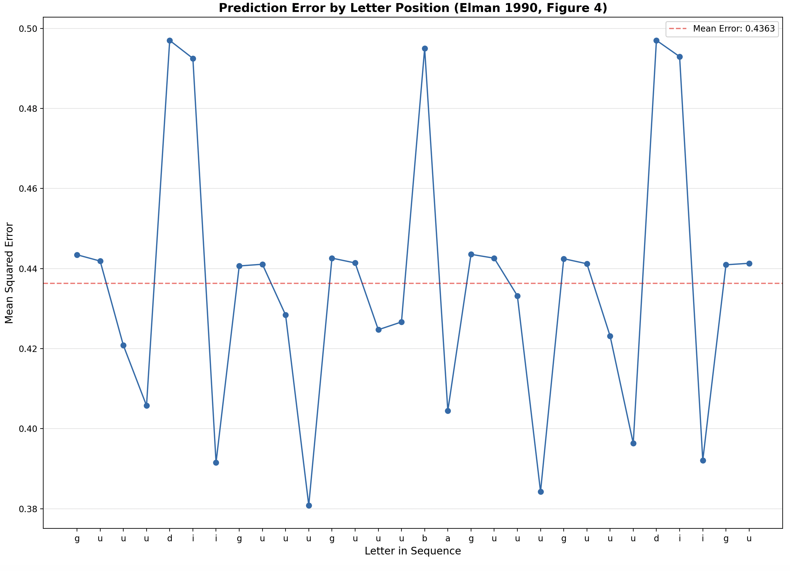
The cv_task() gives a couple of different outputs. One allows you to see the evolution of the hidden units over time. The second allows you to see a graph generated from our own code that mimic’s Elman’s Figure 4 from his paper. In that graph you can easily see that the network has a much higher error rate predicting the consonants – which were added randomly to the sequence. And it has a significantly lower error rate when predicting a vowel. It has learned that specific vowels follow from specific consonants.
Take note of the following steps in the python class. Memorize them and you’ll be able to build most neural networks without any help at all:
In the main() function, you’ll want to make four calls:
1. Create the network.
2. Generate the data (or massage it to fit the needs of the model).
3. Train forward.
4. Train backward.
5. Test using the trained model.
Variations in Network Structure and Input.
To really understand how the network learns and what its limitations are, you’ll need to vary the training parameters and the input. Here are some experiments to try.
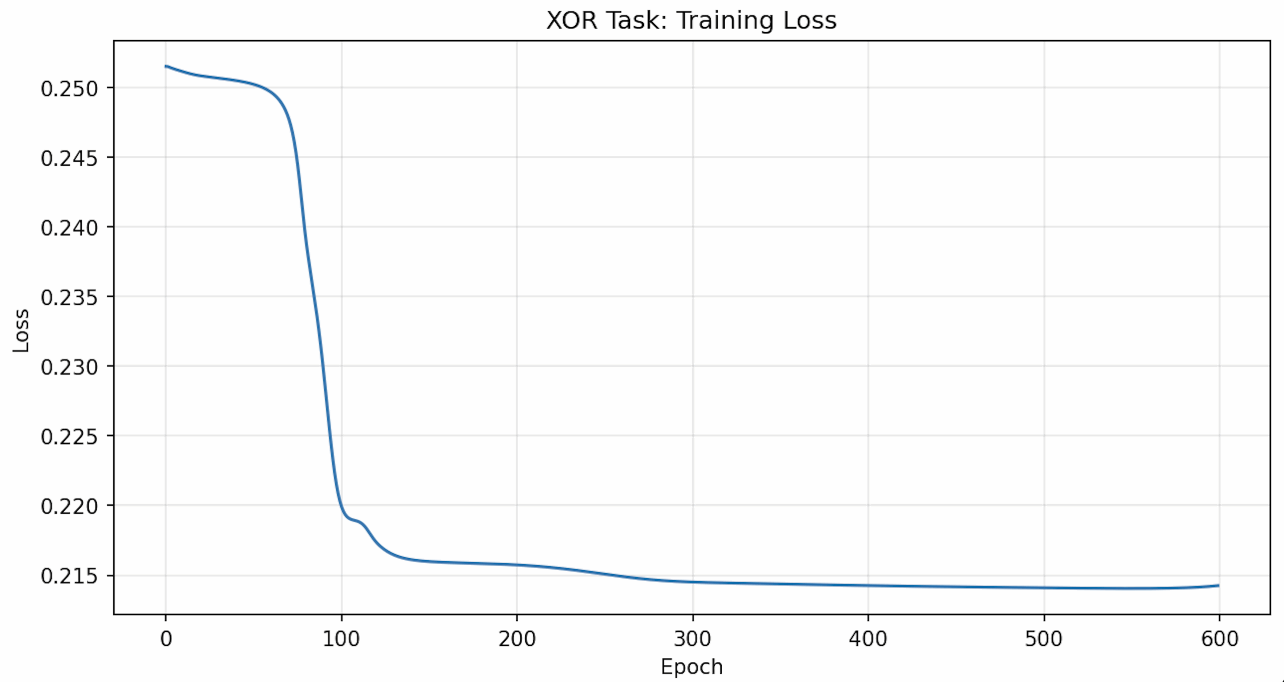
1. For the XOR trial, Elman used a sequence length of 3000 and a total of 600 epochs of training. This results in the following type of training loss graph: You should be able to replicate this. The graph shows that we reach a minimum loss shortly after 100 epochs. Set the number of epochs to 100 and see if this is true.
2. The Console output of the elman_network_complete.py code shows a table comparing the predicted and actual values for the first 20 positions of the input sequence.
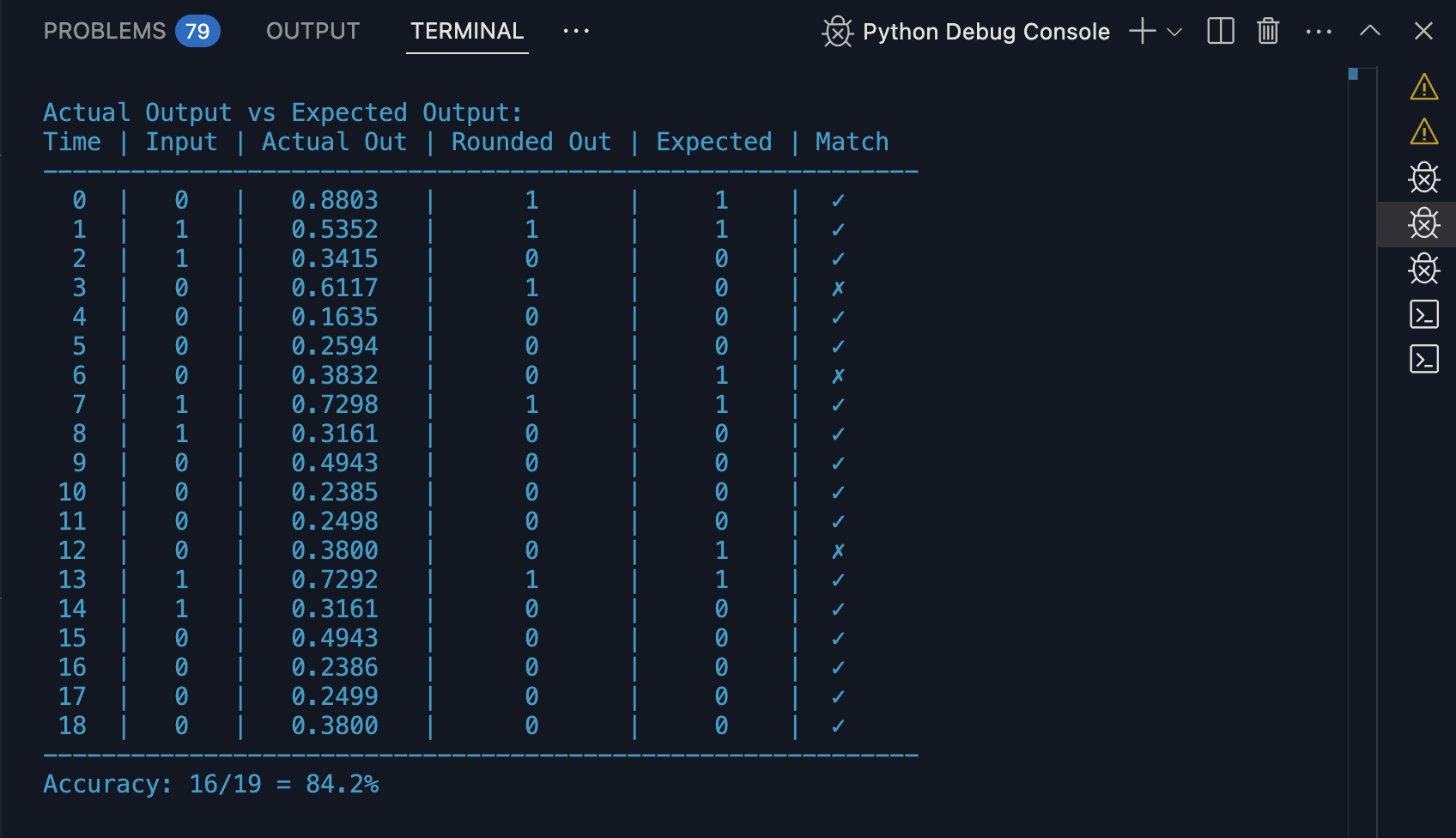
Notice that the ‘Actual’ out is predicting the value at the NEXT time index in each row. That’s because it’s a prediction. Uncomment the code under the title "Test predictions of the third bit only."
Uncomment from the line ‘# correct = 0’ through the about 16 lines later that says: ‘# print()’ and run again. You will see an additional table in the console that shows the error rates for the XOR rows only.
3. Do it once more for the additional hidden function: Uncomment from ‘#position_errors = [0, 0, 0]’ through ‘# print()’. And run again. This time you will see something that Elman showed in his Figure 3: A table with actual error rates for all the three positions. With this you can clearly see that the network can predict the XOR values easily. But it can’t (and shouldn’t be able to ) predict the other two positions very well. Increase the number of tests from the default 20 if you need to.
4. Notice that when we are done training the network and we then call predict_sequence to put the newly trained network to work, we reset the context. And then in predict_sequence we reset_context() after each prediction. Why do we do that? What happens to the preditions if we don’t reset the context?
5. What if you used 3 hidden units for the XOR tests? Would it still work?
6. What if you used 20 hidden units for the XOR tests? Would you have a loss graph that didn’t require at least 100 training epochs to reach the lower plateau?
Steps To Memorize
Memorize these 4 calls and you are almost done.
Memorize the following and you’ll be able to walk into any neural network talk and understand it better than 99% of the people in the room:
1. Create the network.
a. Init with a learning rate, with weights and biases. In the RNN case, init the context with zeros.
b. Define functions for calculating the sigmoid and the sigmoid derivative.
2. Generate the data (or massage it to fit the needs of the model).
a. In this case, we generated the training sequence.
3. Train. Break it down into 4 pieces.
a. The outermost piece: loop through all the epochs one at a time. Generally it is difficult to circumvent a loop here. One step for each ‘epoch’ or input piece of data.
b. The next piece: One training step. The step calls the forward and the backward training steps and updates any variables such as the context.
c. The forward training step.
d. The backward training step.
4. Test.
Date
December 16, 2025