

Elman’s Recurrent Neural Network

The Recurrent Neural Network.
Introduction: Understanding RNNs
The Architecture (with 4 hidden units)
Forward Pass: Concrete Example
Why RNNs Work: The Key Insights
Section 2. Structure in Letter Sequences
Section 3. Discovering the Notion “Word”
Section 4. Discovering Lexical Classes from Word Order
Section 5. Types, Tokens and Structured Representations.
In Conclusion: What did Elman find?
1. Foundational RNN Architecture
2. Proof of Concept for Learning Structure
3. Influenced the Connectionist vs. Symbolist Debate
4. Inspired Later RNN Architectures
5. Impact on NLP and Sequence Modeling
6. Distributed Representations Insights
Introduction
Jeffrey Elman’s Cognitive Science paper titled “Finding Structure in Time” contains one of the first descriptions of Recurrent Neural Networks (RNNs). And because of this, it is one of the most important papers in the development of AI. We review that paper in detail elsewhere. Here we will take a tour of a simple RNN. We will go through several rounds of forward and back propagation with numbers. This will help you fully understand how RNNs work and why they are still important. If you wish you can go to my third article on the topic, where I show you how to implement an RNN in python.
Here we will use multiple diagrams, code and even some animations to make your understanding as clear as possible with the smallest amount of time. With that: Here are the goals of this review:
Goal
Introduction
The goal is to thoroughly understand the structure of Recurrent Neural Networks — RNNs. RNNs are the basis of all ‘predict the next word’ type of neural network. And at the time of this writing, in late 2025, everyone everywhere is familiar with this form of computation simply by looking a redictive text on their phone. Understanding this type of neural network is critical to understanding all kinds of modern neural networks.
The Problem RNNs Solve
Imagine you’re writing a function to predict the next character in a sequence. Given “hell”, your function should output “o” (to complete “hello”). This seems simple, but consider the problem in this python pseudocode:
def predict_next_char(sequence):
    # How do you write this?
    # The answer depends on remembering EVERYTHING that came before
    return next_char
The challenge you face is this: the next character depends on context that could be arbitrarily far back in the sequence. Compare this to more traditional functions that process inputs independently – they’re stateless. Like the above python pseudocode: You are presenting a single variable to the function that contains all the sequence. But language, music, stock prices, and many real-world phenomena are sequential – what comes next depends on what came before.
Enter Recurrent Neural Networks (RNNs): They’re functions that maintain state across inputs. Think of them as functions with memory. Or think of them as functions meant to process serialized input.
A Simple Mental Model
If you’ve written a state machine, you already understand the core concept:
state = initial_state for input in sequence:
    state = update_function(state, input)
    output = compute_output(state)
An RNN is essentially this, but with two key differences:
1. The update_function and compute_output are parameterized by weights
that are learned from data
2. The state is a vector of real numbers, not discrete states
That is your mental model: A vector of real numbers.
And in fact the Elman network is only slightly more complicated than this mental model.
And if you already are thinking that we can’t possibly hold the state of anything practical in this kind of mental model, you would be correct to think so. There are drawbacks to such a simple model. We will get to that.
Let’s begin to look at how a real Elman network resembles this mental model. To do this we will consider three things: The units, the weights, and the bias terms.
The Architecture (with 4 hidden units)
Here’s what we want it to look like:
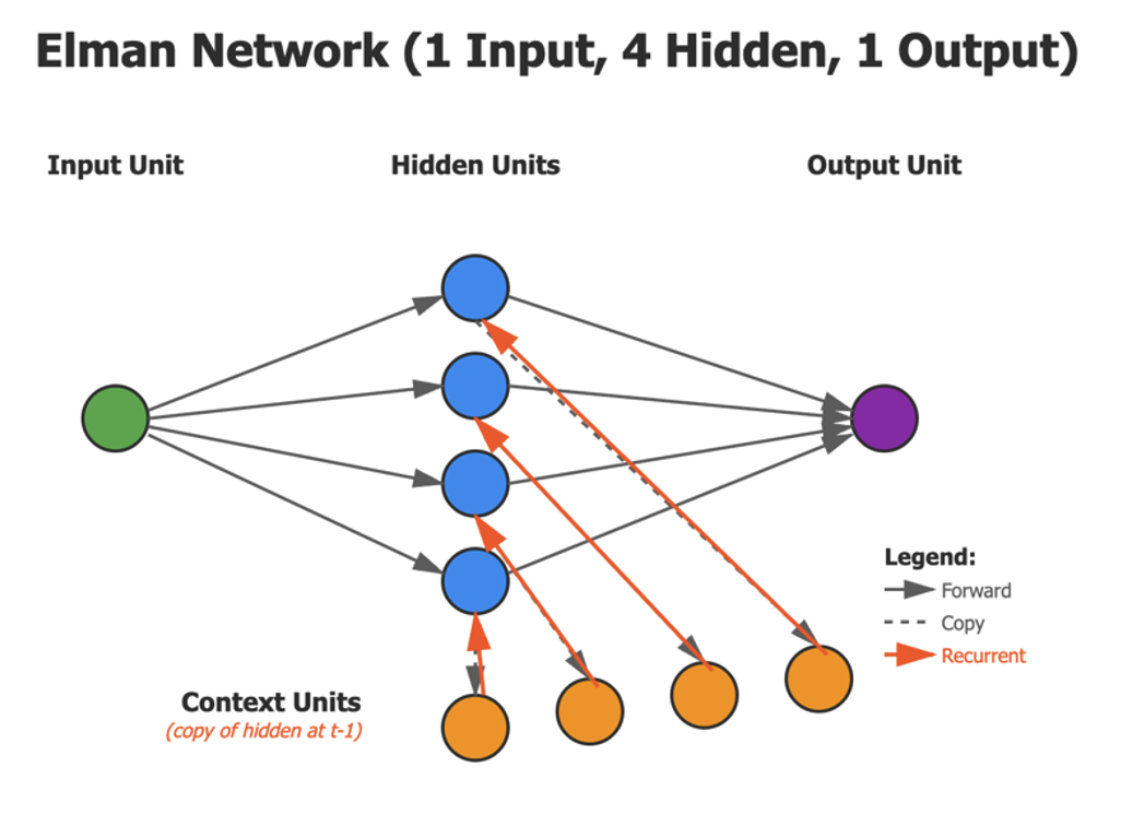
The Units
Let’s build that simple RNN with 4 hidden units. You can see from the drawing that it has one green input unit. In Elman’s paper, the first example involves sequentially feeding a series of zeros and ones into the network. This green input unit is the source of that series of zeros and ones.
The input unit feeds its values into the 4 blue hidden units. These are called ‘hidden’ because they don’t directly interface with the outside world. The green input unit and the purple output unit do that. Those units are therefore not hidden.
In this network drawing you can also see 4 orange context units. These units have a ‘memory’ of the previous state of the hidden units. Each time the output is calculated, the network is reset, and the context units are given the values of the hidden units. They store those values in order to influence the next round of input. Because they store values, they give rise to recurrence of a previous state. They are the reason why the network is called recurrent.
Now let’s fill in the details of what we just described. To build the network in the above diagram, let’s put together an inventory sheet. Here is what we need:
Input Layer:     1 unit  (receives one number at a time – but this may be
                   from a series of 1000 values - just used one at a time.)
Hidden Layer:    4 units (the "state" or "memory")
Context Layer:   4 units (copy of previous hidden state)
Output Layer:    1 unit  (prediction)
Key Insight:
During the forward phase of training, the hidden layer receives input from two sources, the input layer AND the context layer. The input layer provides data depending on the environment. It might be a series of binary values. The context layer provides input that is a copy of the previous values of the hidden layer. In other words, the input the hidden layer receives at time t comes from
1. The current input at time t
2. A copy of itself from time t-1 (stored in context units)
This is how memory works – the past influences the present.
But we haven’t yet described the whole network. Between each layer are arrays of weights. These weights influence the value of the hidden layer. And these weights ALSO are changed during the back propagation phase of training. Let’s add the weights to the diagram and then show what they mean mathematically: 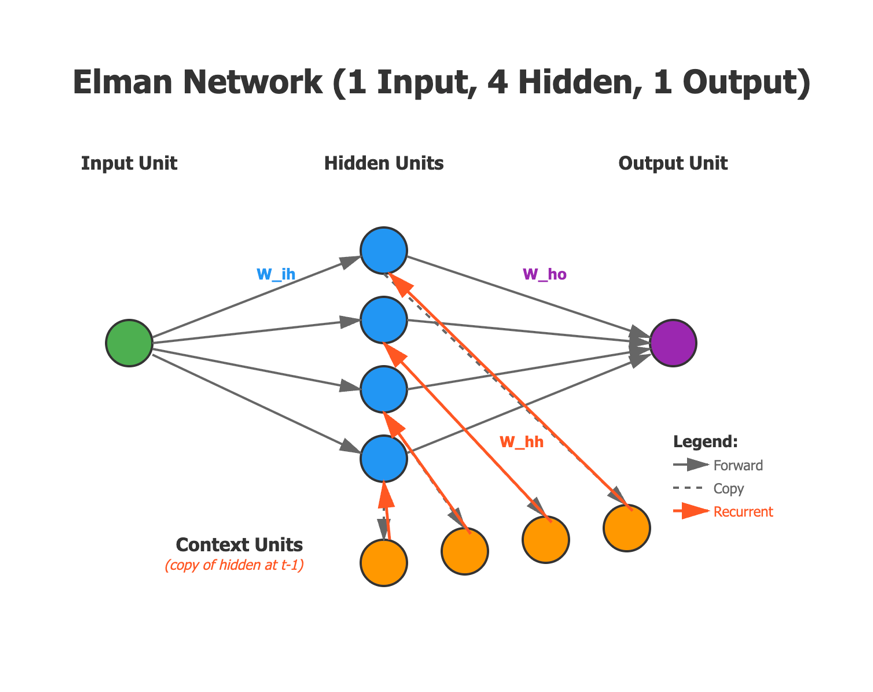
The Weights
We need three sets of weights (matrices). There is one array of weights between the input unit and the hidden units. In our diagram we have one input unit and four hidden units, so that array would be a 1X4 array of weights. Keep in mind that this entire network is designed to handle serial input. So the input will always consist of one value at a time. Thus the size of the input array is always a 1X1 matrix.
However, there may be more than 4 units in the hidden layer. Let’s say there are 16 units. Then the size of the weights array would be 1×16. This is necessary because to multiply the input array (1X1) by the weights array and have a result that is the size of the hidden array (1X16), the weights array must be of size 1X16. If you are having any issue with this logic, see my other papers on Math for Deep Learning I or II.
In the diagram we call the weights array ‘W_ih’ to show that it is an array of weights between input and hidden units.
Next we have an array of weights between the context units and the hidden units. This array we call ‘W_hh’ to show that it is an array of weights between orange hidden (context) units and the blue hidden units.
In this case we have 4 hidden units and 4 context units. Since the context units must store the values of the hidden units from the previous round of learning, the number of context units will always equal the number of hidden units.
And because we multiply the values of the context units by the values in the W_hh weights array to get to the next round of hidden values, the size of the W_hh weights must be 4X4.
Next note that we do NOT have an array of weights going the other direction, from the blue hidden units and toward the orange hidden units. That’s because after each output the values in the blue hidden units are copied without any weighted change directly to the orange context units.
Finally note that we have an array of weights between the blue hidden units and the purple output unit. This array is called ‘W_ho’ to show that it is an array of weights between the hidden units and the output unit. What do you expect the dimensions of the W_ho weights array to be? They must allow us to multiply the hidden units by the weights to obtain the output value. So in our case, this dimension must be 1X4.
Again let’s fill in the details of what we just described and put together an inventory sheet of the weights.
Here is what we need:
W_ih: Input → Hidden (shape: 4×1, so 4 weights) How much each input value affects
      each hidden unit
W_hh: Context → Hidden (shape: 4×4, so 16 weights) How the previous state affects
      the current state (the recurrent connections)
W_ho: Hidden → Output (shape: 1×4, so 4 weights) How the hidden state produces
      an output
But we still haven’t described the whole network. We have to include the bias terms.
The Bias Terms
As I said earlier the weights of the hidden layer were calculated using the values of the inputs and values from the context layer. These values were multiplied by the values in the weights. But there is always one more term in the equation to calculate the hidden layer, and that is the bias term. Here’s a preview of the calculation – which we will examine again later. But I show you now so you can begin to understand how the bias terms fit in.
The formula is this: h_t = tanh(W_ih * x_t + W_ch * c_t + b_h) It’s important to remember this is called the activation function. This particular activation function converts the terms in the parentheses on the right to a value between -1 and 1 using the hyperbolic tangent function tanh.
(Other types of activation functions output values between -1 and 1 or between 0 and 1. Activation functions play an important role in all of machine learning and if this is your introduction to them, keep in mind that
although they have small and important differences, they all reduce our input to an output in a narrow range typically between -1 and 1 or similar.)
Notice the three terms on the right:
W_ih * x_t – this is the contribution from the input and the input-to-hidden weights.
W_ch * c_t – this is the contribution from the context and the context-to-hidden weights.
b_h – this is the bias term.
The formula says that the hidden layer at time t (h_t) is equal to the tanh value of the sum of three terms: (1) The input layer at time index t (x_t) times the weights in W_ih, plus (2) the context layer at time t (c_t) times the weights in W_ch, plus (3) the bias terms. And to drive this fact home: The context layer at time t is the same as the hidden layer at time t-1.
After all that, here are the bias terms. There are 5 total: one for each of the four hidden units, and one for the output unit.
b_h1, b_h2, b_h3, b_h4, b_o
Summary of the Architecture
Let’s put together everything we have seen so far. But let’s consider only the ‘learnable’ values. These are the values that will change during the network training. And these values include the weights and the biases. The other values of the network – the input values, the hidden values, the context values and the output values do, in fact, change. But they change in a fixed way that depend on the input and training.
So here are the total learnable parameters:
Total parameters:
4 (W_ih),
16 (W_hh),
4 (W_ho),
4 (b_h1-b_h4),
1(b_o)
= 29 learnable values.
Forward Pass: Concrete Example
Let’s walk through exactly what happens when we process a sequence. We’ll use small, round numbers only because that will make the math easier to follow. At the end of this article, we’ll link to a complete description of how to implement the Elman network in code.
Initial Setup
Weights (initialized randomly, but we’ll use simple values):
W_ih (Input to Hidden):
[0.5  0.3  0.8  0.2]

W_hh (Context to Hidden, 4×4 matrix):
[0.1  0.2  0.0  0.1]
[0.3  0.1  0.2  0.0]
[0.0  0.2  0.3  0.1]
[0.2  0.0  0.1  0.2]

W_ho (Hidden to Output):
[0.4  0.3  0.5  0.2]

Biases:
b_h = [0.1, 0.1, 0.1, 0.1]  (for hidden units)
b_o = [0.0]                   (for output)
Initial context (t=0):
context = [0.0, 0.0, 0.0, 0.0] (no previous state yet)
Time Step 1: Input = 1.0
The input could be any value. It could be the first value in a series of 2000 bits and be either 0 or 1. Or it could be a matrix itself.
But for these demo purposes it is a single scalar value that happens to be 1.0.
Step 1a: Compute input contribution to hidden layer. The input is 1.0. The weights are 0.5, 0.3, 0.8 and 0.2:
input_contrib = W_ih × input
              = [0.5, 0.3, 0.8, 0.2] × 1.0
              = [0.5, 0.3, 0.8, 0.2]
Step 1b: Compute context contribution to hidden layer. In the very first step, the context doesn’t have any memory of what happened previously. So the contribution of the context to the hidden layer is appropriately zero:
context_contrib = W_hh × context
                = W_hh × [0, 0, 0, 0]
                = [0.0, 0.0, 0.0, 0.0]  (no memory yet)
Step 1c: Combine and add bias. This step is called the linear transformation. It is the combination of the weighted sum of the inputs plus the bias. The result of this is used in the activation function described above.
hidden_input = input_contrib + context_contrib + b_h
             = [0.5, 0.3, 0.8, 0.2] + [0.0, 0.0, 0.0, 0.0] + [0.1, 0.1, 0.1, 0.1]
             = [0.6, 0.4, 0.9, 0.3]
Step 1d: Apply activation function (sigmoid). Above we used a different activation function, namely tanh. Here we use another common activation function, known as sigmoid. The tanh function produces an output between -1 and 1. The sigmoid function produces an output between 0 and 1. In this step we complete the calculation of the values of the hidden layer:
sigmoid(x) = 1 / (1 + e^(-x))

hidden[0] = sigmoid(0.6) = 0.646
hidden[1] = sigmoid(0.4) = 0.599
hidden[2] = sigmoid(0.9) = 0.711
hidden[3] = sigmoid(0.3) = 0.574

hidden_state = [0.646, 0.599, 0.711, 0.574]
Step 1e: Compute output. With the values of the hidden layer for the first forward pass complete, we can calculate the value for the very first output. This is a combination of the values in the hidden layer, the weights to the output, and the bias value for the output:
output_input = W_ho × hidden + b_o
             = [0.4, 0.3, 0.5, 0.2] · [0.646, 0.599, 0.711, 0.574] + 0.0
             = 0.4×0.646 + 0.3×0.599 + 0.5×0.711 + 0.2×0.574
             = 0.258 + 0.180 + 0.356 + 0.115
             = 0.909

output = sigmoid(0.909) = 0.713
Step 1f: Update context for next time step. We have our output, and we haven’t yet described the first back propagation training step. But before we do that, we are going to ‘remember’ the values of the hidden layer by storing them in the context layer:
context = hidden_state = [0.646, 0.599, 0.711, 0.574]
Summary after t=1:
• Input: 1.0
• Hidden units: [0.646, 0.599, 0.711, 0.574]
• Output: 0.713
• Context stored: [0.646, 0.599, 0.711, 0.574]
Time Step 2: Input = 0.0
Now the context has information from the previous time step!
Step 2a: Compute input contribution. The previous input was a ‘1.’ The current input is a ‘0’:
input_contrib = [0.5, 0.3, 0.8, 0.2] × 0.0
              = [0.0, 0.0, 0.0, 0.0]
Step 2b: Compute context contribution. This is where the magic happens – the network “remembers” the previous input! On the first round of training the context had no values and thus no real contribution to the hidden layer. But on the second and subsequent training steps, it makes a real contribution:
context = [0.646, 0.599, 0.711, 0.574]
W_hh (Context to Hidden, 4×4 matrix, same as above):
[0.1  0.2  0.0  0.1]
[0.3  0.1  0.2  0.0]
[0.0  0.2  0.3  0.1]
[0.2  0.0  0.1  0.2]

For hidden unit 0:
  0.1×0.646 + 0.2×0.599 + 0.0×0.711 + 0.1×0.574 = 0.242

For hidden unit 1:
  0.3×0.646 + 0.1×0.599 + 0.2×0.711 + 0.0×0.574 = 0.396

For hidden unit 2:
  0.0×0.646 + 0.2×0.599 + 0.3×0.711 + 0.1×0.574 = 0.390

For hidden unit 3:
  0.2×0.646 + 0.0×0.599 + 0.1×0.711 + 0.2×0.574 = 0.315
The contributions from the context to the hidden layer are now significant:
context_contrib = [0.242, 0.396, 0.390, 0.315]
Step 2c: Combine and add bias. In this step, like before, we are calculating the linear transformation of the hidden layer. Notice that the input didn’t contribute anything at all; but the context layer made a significant contribution. But consider this more deeply: The context is remembering the ‘1’ that was input the first time through. But the new input is a ‘0.’ So the context is actually contributing a memory that is different from the input! But this is what we want: We want a contribution from a ‘memory’ even when that contribution is different from the current input:
0.315] + [0.1, 0.1, 0.1, 0.1]
= [0.342, 0.496, 0.490, 0.415]
Step 2d: Apply sigmoid. As above, we calculate the hidden layer values using the sigmoid activation function. And now we have the hidden layer in step 2.
hidden[0] = sigmoid(0.342) = 0.585
hidden[1] = sigmoid(0.496) = 0.621
hidden[2] = sigmoid(0.490) = 0.620
hidden[3] = sigmoid(0.415) = 0.602

hidden_state = [0.585, 0.621, 0.620, 0.602]
Step 2e: Compute output. We calculate the output by multiplying the hidden layer by the output weights. Notice that after the first pass, it was 0.713. And after the second pass, at 0.701, it is lower, but still very close the the value of the first pass.
output_input = 0.4×0.585 + 0.3×0.621 + 0.5×0.620 + 0.2×0.602
             = 0.234 + 0.186 + 0.310 + 0.120
             = 0.850

output = sigmoid(0.850) = 0.701
Step 2f: Update context:
context = [0.585, 0.621, 0.620, 0.602]
Summary after t=2:
• Input: 0.0
• Hidden units: [0.585, 0.621, 0.620, 0.602]
• Output: 0.701
• Context stored: [0.585, 0.621, 0.620, 0.602]
Time Step 3: Input = 1.0
Let’s do one more forward pass. The XOR logic gate dictates that if our first input was 1, and our second input was 0, then the current input here at step 3 must be 1. If our new input is a ‘1’ and the previous output was 0.701, which direction do you expect the new output to go?
Step1 3a-b: Compute contributions. Our W_ih are the same: [0.5, 0.3, 0.8, 0.2].
input_contrib = W_ih × input
              = [0.5, 0.3, 0.8, 0.2] × 1.0
              = [0.5, 0.3, 0.8, 0.2]
input_contrib = [0.5, 0.3, 0.8, 0.2]

context = [0.585, 0.621, 0.620, 0.602]
Calculate the context contribution to each hidden unit:
Contribution to hidden unit 0:
  0.1×0.585 + 0.2×0.621 + 0.0×0.620 + 0.1×0.602 = 0.243

Contribution to hidden unit 1:
  0.3×0.585 + 0.1×0.621 + 0.2×0.620 + 0.0×0.602 = 0.362

Contribution to hidden unit 2:
  0.0×0.585 + 0.2×0.621 + 0.3×0.620 + 0.1×0.602 = 0.370

Contribution to hidden unit 3:
  0.2×0.585 + 0.0×0.621 + 0.1×0.620 + 0.2×0.602 = 0.299

context_contrib = [0.243, 0.362, 0.370, 0.299]
Step 3c-d: Combine to create the linear transformation and apply the sigmoid activation function:
hidden_input = [0.5, 0.3, 0.8, 0.2] + [0.243, 0.362, 0.370, 0.299] + [0.1, 0.1, 0.1, 0.1]
             = [0.843, 0.762, 1.270, 0.599]

hidden_state = [sigmoid(0.843), sigmoid(0.762), sigmoid(1.270), sigmoid(0.599)]
             = [0.699, 0.682, 0.781, 0.645]
Step 3e: Compute output
output_input = 0.4×0.699 + 0.3×0.682 + 0.5×0.781 + 0.2×0.645
             = 0.280 + 0.205 + 0.391 + 0.129
             = 1.005

output = sigmoid(1.005) = 0.732
To answer the question from earlier: The previous input was ‘0’ and the previous output was 0.701; the new input is ‘1’ so which direction do you expect the new output to go? We expect it to go up, of course:
Summary after t=3:
• Input: 1.0
• Hidden units: [0.699, 0.682, 0.781, 0.645]
• Output: 0.732
What Did We Just Compute?
Look at the pattern:
Time | Input | Hidden State (4 units)              | Output
-----|-------|-------------------------------------|-------
  1  |  1.0  | [0.646, 0.599, 0.711, 0.574]       | 0.713
  2  |  0.0  | [0.585, 0.621, 0.620, 0.602]       | 0.701
  3  |  1.0  | [0.699, 0.682, 0.781, 0.645]       | 0.732
Three Observations:
1. At t=2, the second step, the input was 0.0, but the hidden units still changed – they retained information from t=1.
2. At t=3, with the same input (1.0) as t=1, we got different hidden values – because the context was different
3. The network’s response to an input depends on its history!
The hidden units are encoding a compressed representation of “what has happened so far.”
Training: How Weights Update
Now let’s see how the network adjusts its weights to make better predictions.
Suppose we’re trying to learn the XOR sequence where each bit is the XOR of the previous two bits. Take any two bits, such as 1 and 0, and the third bit represents their XOR value: 1. The XOR rule is simple: If the two bits are the same, such as 0 and 0, or 1 and 1, then the output is 0. ‘Same’ yields zero. If the two bits are different, such as 0 and 1 or 1 and 0, then the output is 1. ‘Different’ yields one.
Here’s the XOR truth table:
Input A | Input B | Output
——–|———|——-
0 | 0 | 0
0 | 1 | 1
1 | 0 | 1
1 | 1 | 0
This is exactly what Elman did in the first section of his paper. Hi input was a series of ones and zeros where every pair of values was used to calculate the next value using the XOR rule.
So his input stream started like this:
1 0
And the third value had to be 1 because the first two were different.
1 0 1
So the fourth value had to be 1 because the second and third were different:
1 0 1 1
But the fifth value had to be 0 because the third and fourth were the same:
1 0 1 1 0
And so on:
1 0 1 1 0 1 1 0 1 1
0 1 1 0 1 1 0
And Elman’s question was whether the RNN could remember this and predict the next value. Thus it would be able to construct an ‘XOR’ logic gate. Unfortunately, you can see their is simply a pattern in the binary values: 1,1,0. The pattern is really all the network needs to learn, and then it should be able to predict the next value.
And that was Elman’s question: Can we create a simple neural network that can recognize this pattern and remember it?
In the above text, we went through three forward steps. That was for didactic purposes. In that text, we only considered the forward sense of training.
Now let’s consider the backward ‘correction’ phase. The backward phase is usually called backpropagation. And it generally consists of two steps:
First, calculate how far the output is from the expected answer. This is usually called the ‘loss.’ Loss is the network’s “report card” – it measures performance. A high loss indicates the network is making bad predictions; it doesn’t understand the pattern. A low loss indicates the predictions are close to reality; the network is learning the pattern.
Second, use the loss to update the weights. If increasing the weight makes the loss bigger, then decrease the weight; if increasing the weight makes the loss smaller, then increase the weight!
As the network is trained, the loss will get smaller as the network learns more and approaches closer and closer to the target value.
Elman performed one back propagation step after each forward step. This is one approach. But it’s not the only way. He could havae performed one back propagation for every twenty forward steps. But for now, let’s do what he did and train with one backpropagation step after each forward step.
Example Back Propagation Step
Thus far, the input sequence for our first three steps was this: [1, 0, 1, …].
At t=3, we just processed input=1.0 and output=0.732, but the target (correct answer) was 1.0.
Calculate the Error or Loss:
error = target - output = 1.0 - 0.732 = 0.268
Our network was too low! We need to adjust weights to increase the output.
Backpropagation in Detail
Let’s go through the back propagation step in more detail, working step by step like we did for the three forward propagation steps above. Remember: the learning algorithm asks: “How much did each weight contribute to this error?” Then it adjusts weights proportionally. Imagine that we went through the three forward propagation steps above, and now we are making our first back propagation step.
Step 1: Calculate the loss and determine the ‘delta’ output.
The delta output, represented as δ_output in the text block, is the amount we will use to adjust the weights in the network. In the text block you can see we calculate the δ_output by finding the loss (output minus target) and multiplying it by the derivative of the sigmoid of the output. In this case, the ‘sigmoid_derivative’ is (output * (1 – output)). The bottom line here is that we want to make a correction to the weights of ‘-0.053’ where the negative sign indicates “increase the output.” But we already knew we wanted to increase the output, because the output was 0.732 but the target was 1.0.
In this text block we calculate the δ_output:
output = 0.732
target = 1.0

δ_output = (output - target) × sigmoid_derivative(output)
         = (0.732 - 1.0) × (0.732 × (1 - 0.732))
         = -0.268 × 0.196
         = -0.053
Step 2: Use the δ_output to adjust the weights between the hidden layer and the output. (We called this the W_ho array of weights.)
We will separate this into two parts, 2A and 2B.
Step 2A: Calculate the gradient, or the degree of change, for each member of the weights array in the W_ho array. The word ‘gradient’ is meant to express the severity of the change. It’s used throughout deep learning projects and it’s worth getting a solid understanding of its meaning. The severity of the gradient depends on how far off we were from the target. Obviously, the further off we were – the bigger the loss – the more we have to correct. But the severity of the gradient ALSO depends on the value in the hidden layer. If the hidden layer has a higher value, we need to apply more force to bring it closer to the target. So the gradient for any given member of the weights array is the δ_output times the hidden value. In the next text block, we calculate the gradients:
gradient = δ_output × hidden^T

For W_ho[0] (from hidden unit 0 to output):
  gradient = -0.053 × 0.699 = -0.037
For W_ho[1]:
  gradient = -0.053 × 0.682 = -0.036
For W_ho[2]:
  gradient = -0.053 × 0.781 = -0.041
For W_ho[3]:
  gradient = -0.053 × 0.645 = -0.034
So the gradients for the weights are [-0.037 -0.036 -0.041 -0.034]
Step 2B: Once we have the gradient for each weight, we still need to calculate the new weight. It’s not as simple as subtracting the gradient value from the weight. (But in some cases it could be.) We do want the weight values to change. But sometimes we can change the weight too quickly. Then during the next forward training pass we have a large error in the opposite direction and we have to correct again. If we overcorrect this time we end up in a loop of overcorrections and we never arrive at a suitable value. Therefore, we want to actually control the rate of learning. To do this, we multiply our gradient by a learning rate. This is usually a number less than one. What it means is that we are reducing the correction by the learning rate factor. We will have to go through more training sessions, but we might converge on the correct level of loss more quickly.
Here, let’s use learning_rate = 0.1 and calculate the new weights:
W_ho (Hidden to Output). In the next text block, we use the gradient, the learning rate and the previous hidden value to calculate the new values of the four weights between the hidden layer and the output layer:
gradient = δ_output × hidden^T
weight_new = weight_old - learning_rate × gradient

For W_ho[0] (from hidden unit 0 to output):
  gradient = -0.037
  W_ho[0]_old = 0.4
  W_ho[0]_new = 0.4 - 0.1×(-0.037) = 0.4 + 0.004 = 0.404
For W_ho[1]:
  gradient = -0.036
  W_ho[1]_old = 0.3
  W_ho[1]_new = 0.3 - 0.1×(-0.036) = 0.304
For W_ho[2]:
  gradient = -0.041
  W_ho[2]_old = 0.5
  W_ho[2]_new = 0.5 - 0.1×(-0.041) = 0.504
For W_ho[3]:
  gradient = -0.034
  W_ho[3]_old = 0.2
  W_ho[3]_new = 0.2 - 0.1×(-0.034) = 0.203
All weights increased slightly! That’s what we wanted. It will make the output larger next time.
So far we have adjusted one set of weights – the weights between the hidden layer and the output.
But we have three sets of weights and we must adjust each of them. The next set we will adjust is the set between the input layer and the hidden layer.
Step 3A. First we will determine the δ_hidden values that we will use to adjust each of the weights.
Previously, we found the gradients to adjust the output weights and found these using δ_output. Here we will find the gradients for the input to the hidden layer and we will use a new parameter called δ_hidden. The calculation of δ_hidden depends on the previous gradient and the sigmoid derivative of the hidden layer. You can see the calculation of the four δ_hidden values below.
For example, the calculation of hidden unit 0, the value is a product of
W_ho, δ_output, and the sigmoid derivative of hidden unit 0.
This is 0.4 × (-0.053) × (0.699 × (1 – 0.699)) = -0.0044.
δ_hidden = W_ho^T × δ_output × sigmoid_derivative(hidden)
From above: W_ho (Hidden to Output) = [0.4  0.3  0.5  0.2]
From above: Hidden units after three inputs: [0.699, 0.682, 0.781, 0.645]
For hidden unit 0:
  0.4 × (-0.053) × (0.699 × (1 - 0.699)) = -0.0044
For hidden unit 1:
  0.3 × (-0.053) × (0.682 × (1 - 0. 682)) = -0.0034
For hidden unit 2:
  0.5 × (-0.053) × (0.781 × (1 - 0. 781)) = -0.0045
For hidden unit 3:
  0.2 × (-0.053) × (0.645 × (1 - 0. 645)) = -0.0024

  δ_hidden = [-0.0044, -0.0034, -0.0045, -0.0024]
Step 3B. Once we have those δ_hidden values, we can update the weights W_ih (Input to Hidden).
You can see that the gradient depends on both δ_hidden and the input values. In this case the input value was 1 in each case. We subtract the product of the gradient and the learning rate from the old weight value to get the new weight.
gradient = δ_hidden × input^T
For W_ih[0]:
  gradient = -0.0044 × 1.0 = -0.0044
  W_ih[0]_old = 0.5
  W_ih[0]_new = 0.5 - 0.1×(-0.0044) = 0.5 + 0.0004 = 0.5004
For W_ih[1]:
  gradient = -0.0034 × 1.0 = -0.0034
  W_ih[0]_old = 0.3
  W_ih[1]_new = 0.3 - 0.1×(-0.0034) = 0.3003
For W_ih[2]:
  gradient = -0.0045 × 1.0 = -0.0045
  W_ih[0]_old = 0.8
  W_ih[2]_new = 0.8 - 0.1×(-0.0045) = 0.8005
For W_ih[3]:
  gradient = -0.0024 × 1.0 = -0.0024
  W_ih[0]_old = 0.2
  W_ih[3]_new = 0.2 - 0.1×(-0.0024) = 0.2002
Step 4. Thus far we have updated the weights from two of the three weight arrays. We have one more array of weights to update, which is the array of weights between the hidden layer and the context layer: W_hh. In this case, we will re-use the δ_hidden values that we calculated last time. But this weights array has 16 values. We will only show the changes for 4 of these in the text block:
gradient = δ_hidden × context^T
From above: δ_hidden = [-0.0044, -0.0034, -0.0045, -0.0024]
From above: Context units after three inputs: [0.585, 0.621, 0.620, 0.602]
From above: W_hh (Context to Hidden, 4×4 matrix):
[0.1  0.2  0.0  0.1]
[0.3  0.1  0.2  0.0]
[0.0  0.2  0.3  0.1]
[0.2  0.0  0.1  0.2]

For W_hh[0,0]:
   gradient = -0.0044 × 0.585 = -0.0026
   W_hh[0,0]_old = 0.1
   W_hh[0,0]_new = 0.1 - 0.1×(-0.0026) = 0.10026
For W_hh[0,1]:
  gradient = -0.0034 × 0.621 = -0.0021
  W_hh[0,1]_old = 0.2
  W_hh[0,1]_new = 0.2 - 0.1×(-0.0021) = 0.20021
For W_hh[0,2]:
  gradient = -0.0045 × 0.620 = -0.0028
  W_hh[0,2]_old = 0.0
  W_hh[0,2]_new = 0.0 - 0.1×(-0.0028) = 0.00028
 ... (and so on for all 16 recurrent weights)
 ...
For W_hh[3,3]:
  gradient = -0.0024 × 0.602 = -0.0014
  W_hh[3,3]_old = 0.2
  W_hh[3,3]_new = 0.2 - 0.1×(-0.0014) = 0.2001
Summary of the BackPropagation step:
Let’s summarize the backpropagation calculations – because although we applied the loss correction to three different sets of weights, we did almost the same thing to each set of weights.
What did we do? Here’s the general procedure to calculate new weights:
First: We calculated the loss: δ_output. This was one value. And it was calculated using the difference between the target output and the actual output, as well as the sigmoid_derivative of the output. In our example, the value was -0.053. Later we calculated a new loss, which we called δ_hidden. This depended on the original loss as well as the sigmoid_derivative of the 4 hidden unit values. Both times we are adjusting our loss based on the sigmoid derivative of unit values.
Second: We used the delta values to find the gradients. The gradient is always the delta value times the upstream unit value.
Third: We adjusted the gradient by the learning rate.
Fourth: We adjusted the weight by the gradient. In our case, we increased the weights by adding.
What Did We Learn?
After this single backpropagation training step:
1. Output weights increased – the network will produce a larger output for similar hidden states
2. Input weights increased slightly – input of 1.0 will activate hidden units a bit more
3. Recurrent weights increased – the network learned how to better use its memory
Do this thousands of times with thousands of examples, and the network discovers the patterns in your sequence!
Why RNNs Work: The Key Insights
1. State representation:
The 4 hidden units and the 4 context units encode a compressed summary of the sequence history. With random weights, this is gibberish. After training, each unit learns to track different aspects of the pattern.
2. Recurrent connections:
The W_hh weights determine what information to preserve from the past and what to forget. The network learns which historical features matter for prediction.
3. Gradient descent:
By computing how each weight affects the error, we can adjust all 29 parameters simultaneously to improve predictions.
4. Compositionality:
The network can handle sequences of any length: patterns learned at time t=10 apply at t=1000. We need far fewer parameters to store a pattern than we would need if we were storing separate logic for each time step.
(Link to Medium paper to Implement the Elman RNN.)
Date
December 28, 2025