The Elman paper contains one of the first descriptions of Recurrent Neural Networks (RNNs). And because of this, it is one of the most important papers in the development of AI. Here we will take a detailed tour through his 1990 paper: ‘Finding Structure in Time.’ You should find a pdf copy online and follow along for the best experience. As we go through it, you will see he is using a sequence of values — like boolean values, letters or words – to learn to predict other values in the same sequence. It may strike you that learning a sequence of values is not all that different than learning the nearest values in transformer architecture. And when you understand that, you’ll begin to appreciate the importance of this little publication.

Here we will use multiple diagrams, code and even some animations to make your understanding as clear as possible with the smallest amount of time. With that: Here are the goals of this review:

Goal

Introduction

First We will summarize it paragraph by paragraph like a real journal club would. We will consider the three types of data that Elman used to demonstrate the network. Elman first used sequences of binary values that represented an ‘XOR’ circuit. We wil xplain the ‘XOR’ circuit and how Elman represented it. We will try to understand whether his result was trivial or non-trivial. Second, he asked the network to predict letters from strings of letters, designed in a very specific manner. We will explain what he did, why it might seem peculiar today, and how this peculiarity affects
the results.

And third, Elman used sequences of words and asked the network to predict new words. Again, we will go through the details of his experimental design. And we will ask: How was he limited by his computer resources? We also will link to a separate article where we recreate the Elman network in python, and fully explain how to use it to recreate the Elman experiment.

Throughout, we will use diagrams and code to make the explanation as clear as possible. If there is a broader area of background that you might need, then I will provide links to other articles. With these background works, you will have everything to understand RNNs perfectly clearly.

Examine the Paper

In Jeffrey L. Elman’s publication, ” Finding Structure in Time” in Cognitive Science, 1990, he spends much of the introduction describing what we now call recurrent neural networks – just as we did above. And our depiction of this type of network is purposely meant to be exactly parallel with the depictions given in the paper. So we won’t dwell on the introduction any furthers. Elman has 5 more sections before the Conclusions section. These are divided roughly by the types of data he analyzes with his network:

1. Exclusive-Or. Here he gives a string of binary values to the network and asks the network to calculate the XOR value.

2. Structure in Letter Sequences. Here he asks whether the memory is sufficient for a more complex sequence than XOR. He provided 6 letters consisting of consonants and vowels formed with certain rules. There were represented by 6-bit values. The network was asked to predict the next letter.

3. Discovering the Notion
“Word.” In this section the task becomes still more complex, using letters to form words and asking the network to predict the next letter.

4. Discovering Lexical
Classes from Word Order. In this section, Elman tests whether the network can predict word order. He divides words into classes and found that although the network was poor at finding perfect recall of word order, it could predict word classes: It could learn verbs, and could learn that some require direct objects, while for others the direct object is optional: ‘Mom ate an apple’ and ‘Mom ate’ is an example.

5. Types, Tokens and Structured Representations. In this section he talks about the internal representations of symbols and how these differ in traditional computer systems and PDP (neural network) systems.

Section 1. Exclusive-Or

If you examined the python implementation of Elman’s RNN (link) you will see that it works quite will at the XOR task. It takes in a sequence of numbers and learns the XOR pattern. This is a little magical: We don’t instruct it to remember a pattern, we just feed it ones and zeros. It learns the pattern on its own. This is, I think, what Elman was thinking when he said the RNN was an internal representation of time. The network captures the pattern. Then it gives it back in predictions.

What is actually happening in this section? Elman inputs strings of 3000 bits. He does 600 passes. The bits consist of two 1-bit inputs followed by a third bit that is the XOR value of the previous two inputs, as in this example:

input: 1 0 1 0 0 0 0 1 1 1 1 0 1 0 1

index: 0 1 2 3 4 5 6 7 8 9 10 11 12 13 14

Thus the value at index 2 represents the XOR value of index 0 and index 1. The value at index 5 represents the XOR value of index 3 and index 4. This is NOT a sequence where the value at every index represents the XOR calculation of the previous two values. It is a sequence in groups of 3: Two values followed by their XOR result.

The problem that Elman wants to solve is this: When the network sees an input, it needs to predict what comes next. There appear to be only three different cases:

When the input comes from Positions 0, 3, 6, 9… then predicting the bit at the next position has a HIGH error. It is fundamentally unpredictable. The first two bits in every group of three are random.

When the input comes from Positions 2, 5, 8, 11… then predicting the bit at the next position has a HIGH error. It is fundamentally unpredictable because the first two bits in every group of three are random.

But when the input comes from Positions 1, 4, 7, 10… then predicting the bit at the next position has a LOW error. It is computable as the XOR value if you remember the previous 2 bits.

In different words:

If the network received a ‘0’ as input from index 1 in the above diagram, and it remembers the ‘1’ from index number 0, then the network will correctly predict the value at index 2 to be the XOR of ‘0’ and ‘1’ = 1.

However, if the network received the same values — a ‘0’ as input from index 3, and it remembers a ‘1’ from index 2, then it will incorrectly predict the value at index 4 to be the XOR of ‘0’ and ‘1.’ But the value at index 4 was just a randomly chosen value.

To get the predictions right, the network needs to maintain a wider context – basically tracking “where am I in the 3-cycle?” – not just “what were the previous two bits?”

To make the correct prediction, the network has to have a bigger context. It needs the current input and the previous value. And this is one of the hallmark observations from this paper: Neural networks are better than traditional software at maintaining context. We’ll come back to this point near the end. Elman emphasizes it as well.

Elman measured the error in the network’s predictions as a function of its position in the sequence. The next figure is similar to what Elman presented and shows the crucial fact: The error goes down when the network is in ‘phase’ with the 3-cycle pattern. Every time the next value is the XOR value, the network predicts it with high accuracy.

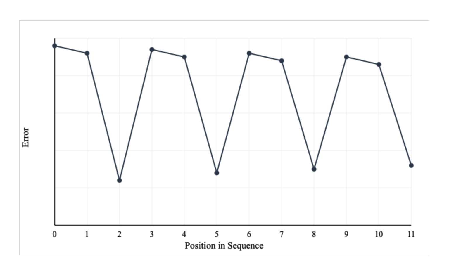
The network struggles to predict positions 0, 1, 3, 4, 6, 7 because they are random. But it can predict every third position — 2, 5, 8 — because this is the XOR position.

That’s why Elman’s graph shows this oscillating pattern – it reveals that some predictions require deeper temporal reasoning than others!

You might sense a difficulty with this strategy: Once the network learns the XOR calculation, it can then apply it to EVERY value and its previous value. If that is all it does, then it will get every third value correct. This is true. But the network has to learn the XOR calculation and store that knowledge. So the network has to hold three things: the input value, the previous input value, and formula for calculating the XOR value. You might object and say: It only has to hole the previous value and the formula for XOR because the current value is the input value. So it’s not all that complicated. Maybe Elman thought the same thing. So he devised more complex tests of the network, starting with looking for structure in letter sequences.

Section 2. Structure in Letter Sequences

In this section, Elman invented a scheme using consonants and vowels to test whether the network can predict the next letter in a string.

The setup is like this:

1. Three consonants – b, d and g – were combined randomly for 1000 letters. This gave a 1000-letter sequence.

2. Then each consonant was replaced using the rules: b = ba, d = dii, g = guuu. This gave 6 characters that could then be represented by 6 bits each. The sequence was then not entirely random. Because each b was followed by an a. Each d was followed by two I’s and so on.

Thus, an initial string of the form “bdgbdg” . . . gave rise to the final string “badiiguuubadiiguuu”.

Since there were 6 characters total, Elman represented each of the 6 characters as 6-bit values in memory. And the basic XOR network from above was expanded to have 6 bit input vectors, 20 hidden units, 6 output vectors and 20 context units.

The training was to present each 6 bit letter, one at a time, to the network. The input vector is therefore a 1X6 matrix. And since there are 20 hidden units, the first set of weights, W_ih, is a 6X20 matrix of weights. And the test was to predict the next input. The network was trained on 200 passes through the sequence of 1000 letters.

The error in predictions oscillated. But the network always had a lower error in predicting that ‘a’ was the letter after ‘b.’ Similarly, it had a lower error predicting ‘i’ was after ‘d’ and ‘u’ was after ‘g.’ Even better: It learned that there were two ‘i’s after d and it was good at predicting two ‘u’s after g. But it was less good at predicting the third ‘u’ after ‘g.’

The author notes the complexity of this result: The network remembers not only that a specific vowel exists after a specific consonant, but also which vowel. And furthermore unlike the XOR pattern, the vowel pattern has different lengths. And the RNN remembers these different lengths: It is in essence predicting not only the next 6 bit character but the next two or the next three in the case of guuu. And the network worked well even though the input consisted of 6-bit patterns instead of the previous 1-bit input.

Elman took it another step further: If it can recognize and predict letters in a string, can it predict words in a sentence?

Section 3. Discovering the Notion “Word”

The author speculates about the relationship between the neural network he has described and the notion of a ‘word.’ He goes on to imagine versions of the network that will form real words from training with other words in sentences. In a very real sense, he is talking about the type of word prediction we have now seen standard above our keyboards in every text messaging app.

To test this idea, Elman created a simulation using a stream of 4,963 letters (encoded as 5-bit vectors) representing 200 sentences concatenated together with no breaks between letters or words.

He used a network with 5 input units, 20 hidden units, and 20 context units was trained to predict the next letter in the sequence.

The illustration I show below is taken from his Table 2:

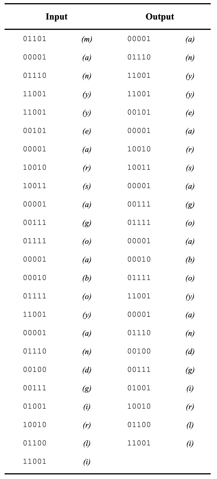
Reading from top to bottom in the Input string, you can see words that form sentences. And on the right you can see what the expected output from the network should be, if it correctly predicts the next letter in the sequence.

After just 10 training passes through the corpus, the network hadn’t memorized everything but had learned something crucial about the structure of the input.

The key finding appears in the error patterns over time: prediction error spikes at the beginning of each new word and decreases as more letters are received and the sequence becomes more predictable. These error peaks effectively mark word boundaries, demonstrating that the network discovered what constitutes a “word” purely from the statistics of letter co-occurrence, without any explicit instruction about word boundaries. While not a complete model of word acquisition (which requires semantic and contextual information), the simulation proves that important cues to linguistic unit boundaries exist in the sequential structure itself, and simple recurrent networks can extract this information autonomously.

Section 4. Discovering Lexical Classes from Word Order

In the final experimental section of the paper, Elman explores whether neural networks can discover abstract linguistic categories (like noun, verb, animate, etc.) purely from word order patterns.

Elman created 10,000 short sentences (2-3 words) using 13 noun and verb categories and 15 sentence templates, generating a stream of 27,534 words with no sentence boundaries. Each of the 29 unique words was encoded as a random 31-bit vector.

The new network had 31 input units, 150 hidden units, and 150 context units. It was trained to predict the next word in the sequence.

The results showed that after six passes through the training sequence, the network couldn’t predict exact words. However, it learned to predict the probability distribution of possible successors with remarkable accuracy—achieving 0.916 cosine similarity with the expected likelihood vectors.

In the setup, Elman created a sentence generation system using 6 classes of nouns and 6 classes of verbs – including categories like NOUN-HUM (man, woman), NOUN-ANIM (cat, mouse), VERB-EAT, VERB-PERCEPT, and a few more.

The 12 noun and verb classes were used to produce templates for sentence generation. The generator then produced 10,000 random two- and three-word sentences composed of these 12 classes. The template might be NOUN-HUM VERB-EAT NOUN-INANIM. And from that template, a sentence was generated. For example: “girl eat bread.” The complexity might seem unnecessary but at that time a formal way of generating the sentences was needed in order to give credence to any prediction of the next word.

The crucial discovery came from analyzing the network’s internal representations. By examining and statistically clustering the hidden unit activation patterns, Elman revealed that the network had spontaneously developed a rich hierarchical category structure: It discovered the major division between verbs and nouns, then further subdivided verbs into transitive, intransitive, and optional-object types. Nouns were organized into animates versus inanimates, with animates split into humans versus animals (further divided into large and small), and inanimates categorized as breakables, edibles, or agentless subjects. These categories emerged purely from statistical patterns of which words could follow which.

A particularly striking demonstration involved introducing a completely novel word “zog” (replacing “man”) without any further training. The network immediately assigned it an internal representation clustered with human nouns, showing it could use distributional cues to infer the “meaning” (or at least the category membership) of unknown words—much as children do when encountering new vocabulary. Elman emphasizes that these categories are “soft” and hierarchical, with graded boundaries rather than rigid distinctions, and that meaning is fundamentally context-dependent—the hidden unit patterns represent not just words but words-in-context. This behavior aligns with the idea that while individual words may be unpredictable, word classes are highly predictable from context.

Section 5. Types, Tokens and Structured Representations.

This section explores how simple recurrent networks handle symbolic representation differently from traditional computational models. Traditional models use discrete symbols with fixed names, whereas PDP networks (neural networks) use distributed activation patterns across hidden units. These distributed representations have a crucial property: they’re context-sensitive, meaning the same word can have slightly different internal representations depending on where it appears. Rather than being a limitation, this context-sensitivity greatly extends the network’s representational power, allowing it to capture both general categories and specific instances simultaneously.

The distributed representation scheme offers significant advantages over traditional approaches where each node, or parameter in a class, represents a single concept. In the network’s hidden units, concepts emerge as patterns across multiple nodes, with each node participating in many different representations. This means a fixed number of analog units can theoretically represent an infinite number of concepts. Although in truth we still don’t use analog representations of units in neural networks. So his statement could be modified: a fixed number of neural network units can represent a large number of concepts. In Elman’s sentence-processing simulations, these hidden units performed double duty—representing both the current input and encoding temporal context for processing future inputs. The network developed representations that captured both word meanings and grammatical categories, which became apparent when clustering analysis revealed systematic organization of the internal patterns.

The network naturally solves the type/token problem without requiring explicit indexing or binding operations. When analyzing all 27,454 word occurrences in the training data, the network distinguished 29 types (different lexical items) while also differentiating individual tokens (specific occurrences of each word). The tokens of a type clustered together but weren’t identical—subtle differences reflected their contexts. For example, instances of “boy” in sentence-initial positions grouped together, as did sentence-final instances, and this same structural pattern appeared for “girl.” Geometrically, the network organized its high-dimensional representational space so that types occupied distinct regions while tokens of the same type were elaborated in parallel, systematic ways based on their contexts.

In Conclusion: What did Elman find?

1. The network learned distributional patterns: After 6 passes through the corpus, the network developed internal representations that captured word order constraints. While it couldn’t predict exact words, it learned which classes of words could follow others.

2. Emergent hierarchical categories: Through clustering analysis of hidden unit activations, the network spontaneously discovered:

Major division between verbs and nouns

Verb subcategories (transitive, intransitive, optional-object)

Noun hierarchy: animates vs. inanimates

Animates: humans vs. animals (large vs. small)

Inanimates: breakables, edibles, and agent-less subjects

3. Context-sensitive representations: The network developed different representations for the same word in different contexts – successfully implementing a type/token distinction without explicit symbolic indexing.

4. Novel word learning: When Elman introduced a novel word “zog” (replacing “man”), the network immediately assigned it an appropriate representation based solely on its distributional behavior, similar to how children infer meaning from context.

The key insight was that abstract linguistic structure can emerge from sequential co-occurrence patterns alone, without pre-specified grammatical categories or semantic features.

Impact

Elman’s 1990 paper had several major impacts on AI development:

1. Foundational RNN Architecture

The Simple Recurrent Network (SRN/Elman Network) became one of the first practical and widely-adopted recurrent architectures. It demonstrated that you could train networks with temporal dependencies using backpropagation, which was a significant breakthrough at the time.

2. Proof of Concept for Learning Structure

The paper showed that networks could discover hierarchical linguistic structure (like part-of-speech categories, verb subcategorizations) purely from distributional patterns – without hard-coded rules or symbols. This was a major argument against the prevailing symbolic AI view that such structure had to be explicitly programmed.

3. Influenced the Connectionist vs.Symbolist Debate

Coming during the heated debates between symbolic AI and connectionism (late 1980s-1990s), Elman’s work provided concrete evidence that neural networks could handle structured, sequential data – something critics like Fodor and Pylyshyn argued was impossible without symbolic representations.

4. Inspired Later RNN Architectures

The Elman network directly influenced:

·
LSTMs (Hochreiter & Schmidhuber, 1997) – which added gating mechanisms to solve the vanishing gradient problem Elman networks suffered from

·
GRUs and other modern RNN variants

·
The general principle of using hidden state as memory became fundamental to all recurrent architectures

5. Impact on NLP and Sequence Modeling

The paper demonstrated that language could be modeled as a prediction task on sequences, which became central to:

·
Statistical language modeling

·
Word embeddings (Word2Vec, which also uses prediction tasks)

·
Modern transformer-based models (which still use next-token
prediction, though without recurrence)

6. Distributed Representations Insights

Elman showed how distributed representations could capture both categorical (type) and contextual (token) information simultaneously – a key insight for understanding how neural networks represent structured information.

The paper was essentially a proof that temporal structure and abstract linguistic knowledge could emerge from simple learning mechanisms – a foundational idea that continues to underpin modern deep learning approaches to sequence modeling.

Date

December 10, 2025

Tags:

Math