Math for Deep Learning II

(Click to jump to section)

Matrix Transformations – The Core Architecture of LLMs is Matrices.

Learning Matrix Transformations is All You Need.

Prerequisites: Multiplying Matrices

Example: Reducing a 10 × 1 Matrix

Transforming, Not Just Reducing

Introduction

Matrix transformations are absolutely fundamental to LLM training – they’re essentially the mathematical backbone of the entire process.

If you want to be ready for the automobile, you have to quit your job at the factory for horse whips. Even if it’s the best whip factory in the world.

That’s what this series is intended to do: Get you ready for the world of AI. Will AI itself start to advance AI? That’s what some are predicting. But if you want to get in the field now, you’ll need to learn the basics.

This is the second article in a series on the basic math you need if you’re working with large language models on your own machine—or if you’re transitioning from traditional development work into AI. But unlike other guides, where the goal is to strictly teach you the math or teach you the machine learning concepts, here we’re focusing on something different: why you need to know this math.

Matrix Transformations – The Core Architecture of LLMs is Matrices.

Weight Matrices ARE the Model

Every learned parameter in an LLM is stored in weight matrices. For GPT-3 with 175B parameters, that’s 175 billion numbers organized into matrices. These matrices transform inputs through layers, where output = activation(input @ Weight + bias). And the transformer – the key innovation in recent LLMs, is pure matrix math.

The bottom line is that without matrix transformations, LLMs wouldn’t exist. They’re not just important – they’re the entire computational substrate. Every “thought” an LLM has is a cascade of matrix multiplications transforming embeddings through learned weight spaces.

This is why linear algebra is considered the most important mathematical foundation for deep learning, and why hardware accelerators (TPUs, GPUs) are specifically designed to optimize matrix multiplication above all else.

Learning Matrix Transformations is All You Need.

In this article, we will learn how to implement matrix transformations. This is not really all you need. But it’s so fundamental, that without it, you’re not in the game.

These transformations come in many types, including rotations, scalings, shearing, reflections, projections and combinations of types that you might have heard of like affine transformations. But these types are all different variations of the same underlying operation.

Let me repeat that: Each listed transformation (rotation, scaling, shear, reflection, projection) is a linear map applied by multiplying a matrix A by a vector x.

And combining multiple transformations into one, which is referred to as composing transformations, can be achieved by multiplying one matrix by another.

An alternative view of the very same operation is to talk about batching, where we collect k input vectors, and arrange them in columns. The collection is a matrix. We can then multiply that by a matrix to achieve the transformation.

Prerequisites: Multiplying Matrices

In Matrix Fundamentals Part I, we talked about the most fundamental exercise with matrices: how to multiply them.

We covered two rules you must remember:

The number of columns of the first matrix must equal the number of rows of the second.
The size of the result is determined by the “outer” dimensions (rows of the first × columns of the second).

We worked through several examples, because this is not just an abstract exercise. If you don’t fully understand matrix multiplication, you won’t get far in AI engineering. It’s that critical.

Goal and Outline

In this article we have two major goals and two minor goal. The first major goals is to impress on you the importance of matrix transformations to LLMs. The second major goal is to get you familiar with the definition and operation called matrix transformation.

The first minor goal is to get you familiar with the variations of matrix transformations that we mentioned above. The second minor goal is to expose you to how mathematcians think about multidimensional space and how they visualize these transformations.

That second minor goal is more important than you might think: One of the greatest difficulities of creating an AI is to understand what’s inside it and how that composition of variables is changed by training. If you start dreaming in 170 billion dimensions, then you are on your way to getting hired by a major AI firm.

From Tall Vectors to Scalars

First, we’ll use matrix multiplication to learn how to collapse a higher-dimensional matrix into something smaller.

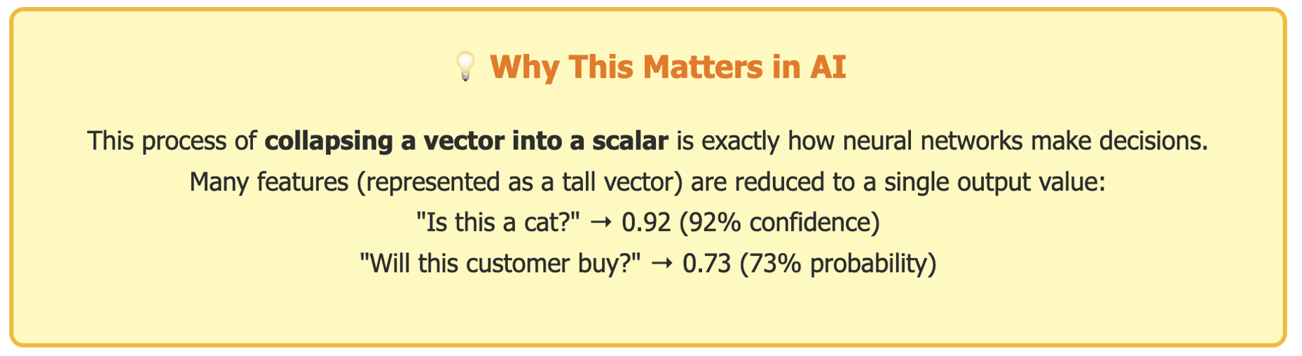
Is this a matrix transformation? You bet. It’s a simple case. But it’s also very important in many LLM models. For example, all models that are trained by a series of cat photos and then asked to decide whether a test image is ‘cat’ or ‘not cat.’ The answer is either true or false. It’s a single number, either 1 or 0.

To produce that single number, a matrix of probabilities is pushed out of the LLM, and the final array of probabilities has to be transformed to a single number.

That’s what we are doing in this exercise.

For example, suppose we want to collapse a (64 × 1) matrix into a (1 × 1) matrix—just a single number.

How do we do that? Simple: we multiply our column vector (64 × 1) by a row vector (1 × 64).

The inner dimensions (64 and 64) match, so the multiplication is valid.
The result has the outer dimensions (1 × 1), which is a scalar.

To keep the math diagrams small, let’s work with a 10 X 1 matrix instead of a 64 X 1 matrix:

Example: Reducing a 10 × 1 Matrix

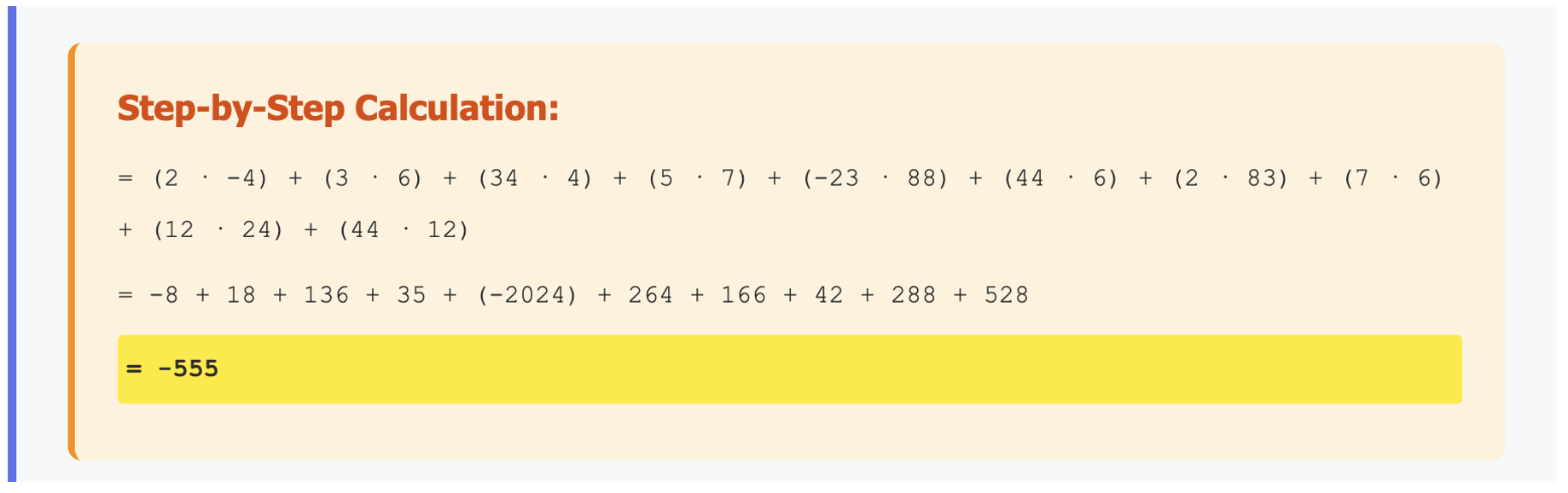
We multiply a (10 × 1) matrix by a (1 × 10) matrix:

If you understood the first article, this should feel straightforward: we’re just applying the same multiplication rules. But notice how this process collapses a 10-element vector into a single number.

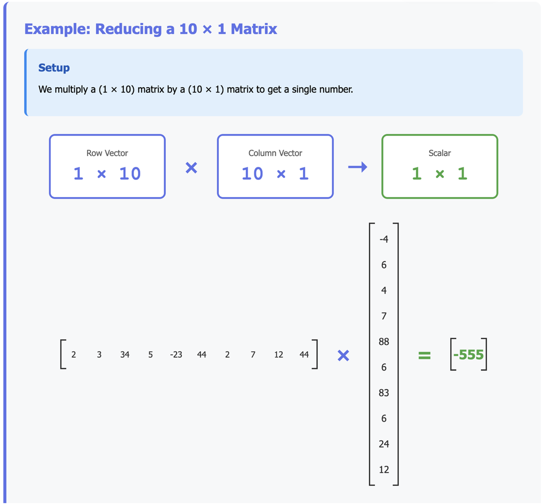
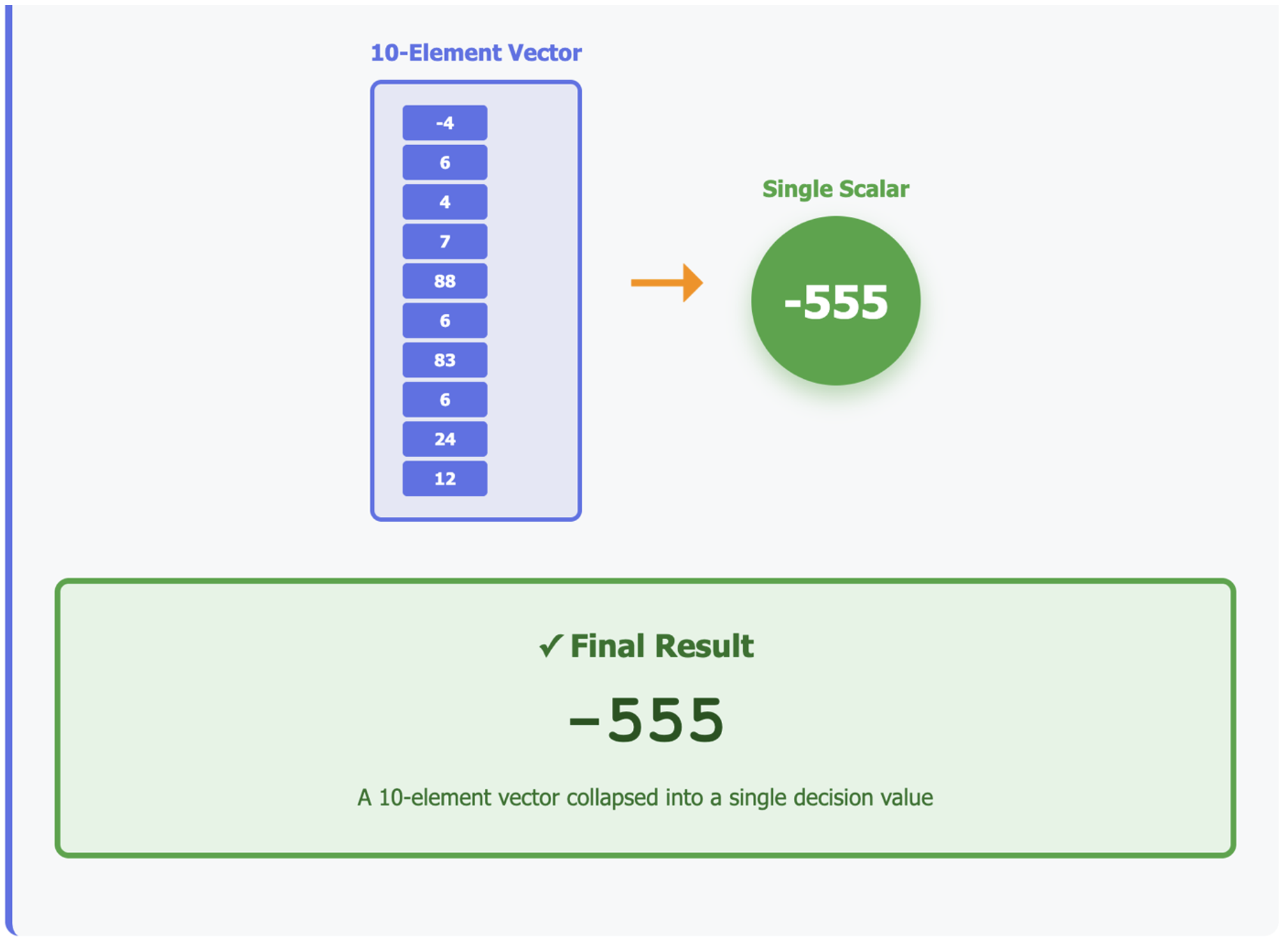
In AI, this is how you might reduce many features into a single decision value.

Transforming, Not Just Reducing

The previous example reduced a vector to a scalar. But what if we start with a rectangular matrix, say (4 × 3)?

If we multiply it by a (1 × 4) matrix, the result is (1 × 3).

This doesn’t reduce the dimensionality—it’s still a 2D matrix—but it transforms the data.

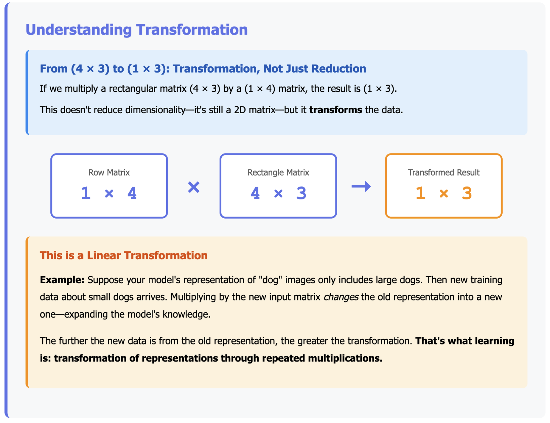
Why is this important? Because transformation is at the heart of training AI models.

This kind of multiplication is called a linear transformation.

Think of it this way: suppose your model’s current representation of “dog” images only includes large dogs. Then along comes new training data about small dogs. Multiplying by the new input matrix changes the old representation into a new one—expanding the model’s knowledge.

The further the new data is from the old representation, the greater the transformation. And that’s what learning is: transformation of representations through repeated multiplications.

Linear Transformations

A matrix transformation is a linear transformation because it satisfies the two fundamental properties of linearity: additivity and scalar multiplication. Work this with me:

The Two Defining Properties of Linearity

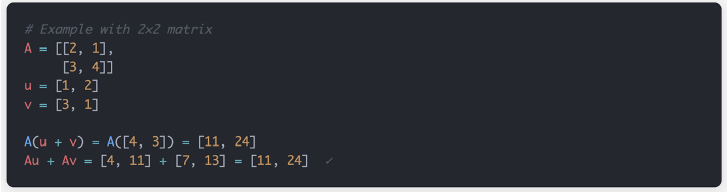
1. Additivity (Preserves Addition)

If you transform the sum of two vectors, you get the same result as summing their individual transformations.

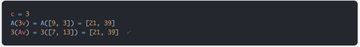
2. Homogeneity (Preserves Scalar Multiplication)

Scaling a vector then transforming it gives the same result as transforming then scaling.

What This Means Geometrically

Linear transformations have special geometric properties:

Preserve Origin:

T(0) = 0 always (the origin stays fixed)
Why: T(0) = T(0·v) = 0·T(v) = 0

Preserve Lines:

Straight lines remain straight (never curve)
Parallel lines remain parallel
Ratios of distances along lines are preserved

Examples:

Rotation: Linear ✓
Scaling: Linear ✓
Shearing: Linear ✓
Translation: NOT linear ✗ (moves origin)
Squaring coordinates: NOT linear ✗ (T(v) = [x², y²])

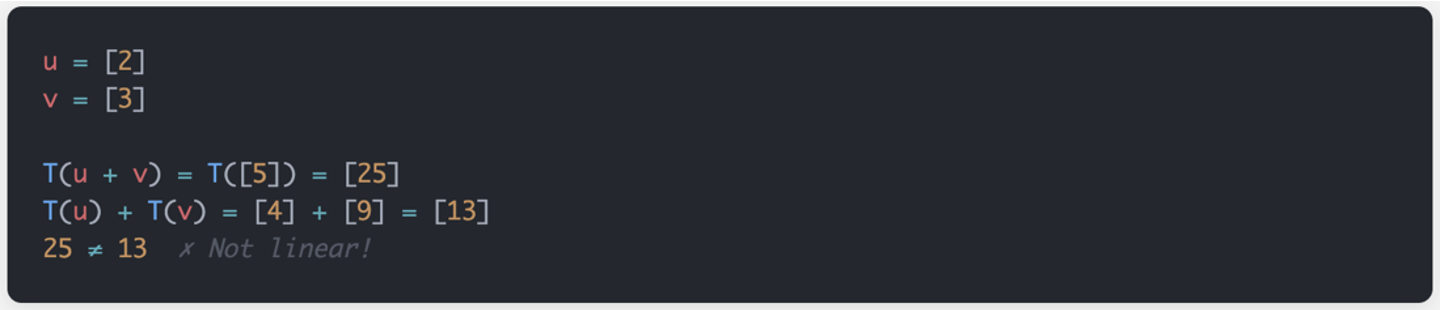
Non-Linear Operations Aren’t Matrix Transformations

If we transform all the values in a matrix by squaring them, this is not linear. And it can’t be represented by a matrix multiplication:

In the Neural Network context, both linear and non-linear transformations are needed! Linear parts are the matrix transformations and non-linear parts are the activation functions.

Pure Linear Transformations are Limited:

First, with only linear transformations, multiple linear layers collapse: ABC·v = D·v (just one matrix!). This problem is outside the scope of this article. But it is huge. I’ll have another article in this series just to unravel the linear layer collapse problem.

Second, linear transformations can only model linear relationships. As mentioned: A single linear transformation can’t represent squares or logs or trig functions. Of which there are many. It can only model linear relationships.

Neural Networks Need Both Linear and Non-Linear Transformations:

Linear (matrices): Transform the representation space
Non-linear (activations): Add expressiveness, prevent collapse

Key Insight for LLMs

In transformers, the attention mechanism is actually a linear transformation with dynamic weights.

The weights themselves depend on the input (making it “self” attention), but the final application is still a matrix multiplication – a linear transformation of V. This is why attention alone isn’t enough – we still need the non-linear FFN layers to give transformers their full expressive power!

Rotational Transformations

Let’s consider a few other types of linear transformations, starting with the rotational transformation.

The illustration shows a Rotation Matrix R and how it can be used to transform the blue starting positions by ‘rotating’ them. In the fixed illustration we use a rotation angle of 25 degrees and a magnitude of 1.6x.

Let’s consider a few other types of linear transformations, starting with the rotational transformation.

The illustration below shows a Rotation Matrix R and how it can be used to transform the blue starting positions by ‘rotating’ them. Try adjusting the angle and magnitude using the sliders:

Interactive Rotation Matrix Transformation

Rotation Angle: 25°

Matrix Magnitude: 1.6x

Rotation Matrix R
[1.449 , -0.677]
[0.677 , 1.449]

● Blue points: Original positions | ● Red points: Rotated positions

━ Blue grid: Original coordinate system | ━ Red grid: Rotated coordinate system

Notice how adjusting the sliders changes both the rotation matrix values and the transformed positions. When magnitude is 1x, points maintain their distance from the origin while rotating. When angle is 0°, changing magnitude scales points along their original direction.

The figure can be dynamically adjusted. If that feature is not available in this publication, download the html from github gist and open it in a browser. Then play with the angle and magnitude. Notice that if you set the magnitude to 1x, then move the rotation angle, the blue dots don’t change their distance from the origin but rotate around it. Then notice that if you set the rotation angle to 0, and change the magnitude, this changes the distance from the origin but the points travel on the same line they were on originally.

Affine Transformations

The affine transformation is a matrix transformation operation. Consider the figure:

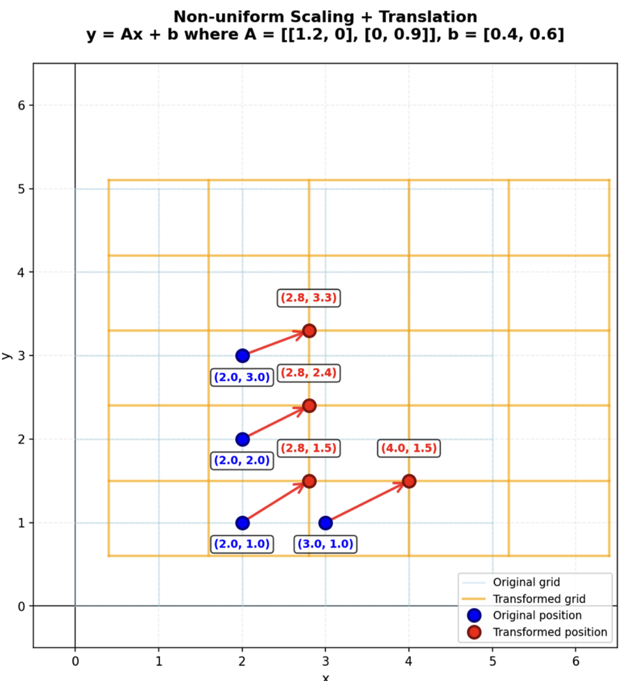
Each blue dot can be represented by a 1X2 matrix.

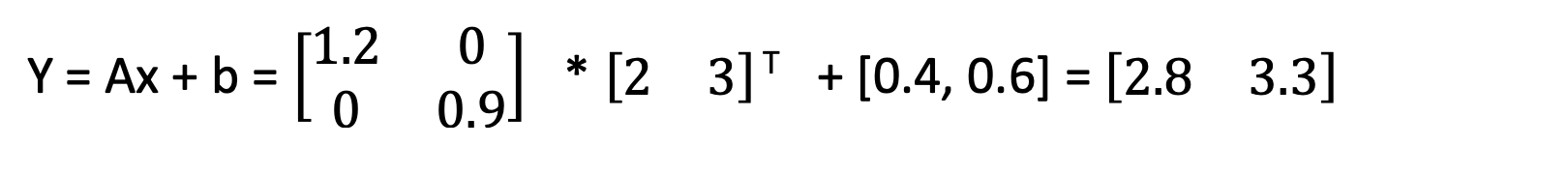
Consider the top-most blue dot and its transformation in space.

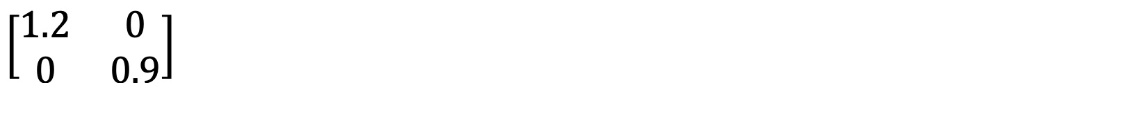
And consider the transformation matrix that does the work:

For that transformation, the formula at the top of the figure can be re-written as:

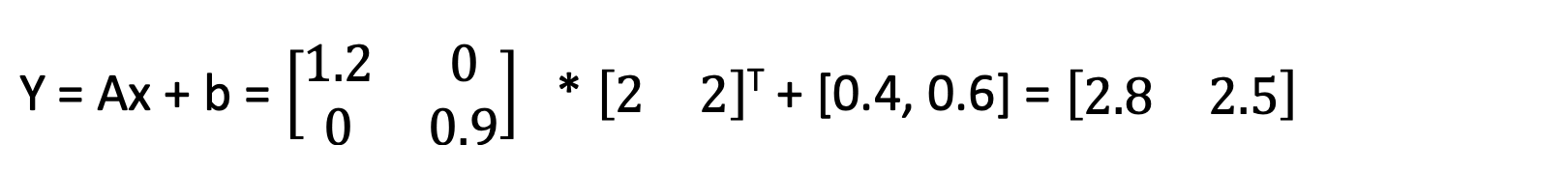
The transformations of the other three blue dots can be written as:

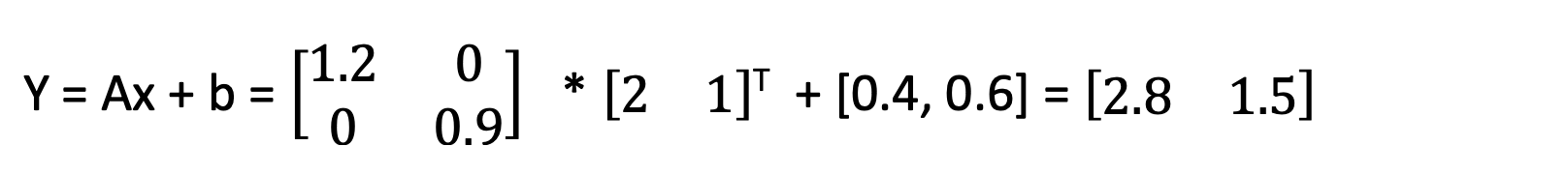
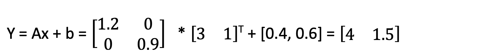
Imagine that each dot has X and Y coordinates. The transforming matrix is matrix A, and that is a 2X2 matrix. Multiplying the 2X2 transforming matrix by the 1X2 blue dot position gives a new 1X2 dot position – the red position.

Look at the background grids. Every blue dot has a position on the blue grid. Every red dot has a position on the orange grid. The light blue background grid consists of nice square shapes. But the orange grid – representing the transformed positions – is shifted to the right and up, and the squares have become rectangles.

That is affine transformation. Straight lines must remain straight. Parallel lines remain parallel. But the entire grid can be shifted or rotated. This illustrates the nature of the affine transformation, or the ‘stretching’ of the positions in at least one dimension.

But the transformation can also result in values that are scaled or ‘sheared.’ It can also be ‘reflected’ or turned back on itself by multiplying by a negative number. And any of these operations can be combined and will still be defined as an affine transformation.

Think about what this means in training a neural network: One can multiply all the values in the ‘hidden’ network and shift or shear their weights. This in turn can essentially change what is being ‘remembered’ by the network. An array representing a ‘C’ chord will be shifted a certain amount when the input array is a ‘G’ chord. This is the process of learning.

The key takeways:

Affine = Linear transformation + translation (bias)
Linear = Just matrix multiplication (no bias)

This takes us back to the formula at the top of the figure: y = Ax + b.

Bottom line: One or more linear operation, when summed together with one bias term, form a single affine transformation on the combined input. An operation without a bias is NOT an affine transformation. It is just a linear transformation.

It’s difficult to understand how these different transformations of existing matrices – or just plain old groups of numbers – work with the relatively small sized matrices in our examples. And so it’s even more difficult to understand what this means when training occurs in an LLM that has billions of parameters. For this reason, the following section is designed to introduce you to some mental modeling techniques that professionals use to understand what is going on in those LLMs. In other words: How do we really understand what is going on in matrices that have an incomprehensibly large number of dimensions?

Visualizing Higher Dimensions

So far, we’ve worked with 2D matrices, but AI models often deal with spaces of hundreds, thousands, or even billions of dimensions. How can we make sense of that and why should we even bother? We need to grasp what this means at least to the degree that we can then model it mathematically. And we need to try to understand what it means to train and refine a model. The truth is that infinite dimensional space is beyond our comprehension. And how it is possible for a billion parameter model to tell us the algorithm for any Leet code problem is also difficult to comprehend. But we can cheat and get a partial view – using some of the following methods.

The Business Approach

One way is to simplify. Mathematicians and data scientists often reduce dimensions by finding the most important ones —“principal components”—and ignoring the rest. This gives us a lower-dimensional picture of the data. Principal Component Analysis – PCA – is one way to achieve this. Many complex scenarios can be modeled in as few as 5 or 6 principal components. Think of it like this: Users of Netflix watch hundreds of movies, but hundreds of thousands are available. In principal component analysis we might find that only 5 movies predict the behavior of a user – if they liked or disliked those five, we can recommend the next movie with high accuracy. Or if they liked a different collection of 6 movies in a different group, we might know that users are very fickle and we can NOT recomment the next movie with high accuracy. Either way, we don’t need to analyze ALL the data. We just need to know the principal components.

The Pure Math Approach

But sometimes, mathematicians don’t visualize at all. They simply accept that we’re limited to three-dimensional intuition, and yet still work comfortably with higher-dimensional spaces. (And yes, dimensions can even be non-integer — “3.4D.”)

A Practical Intuition

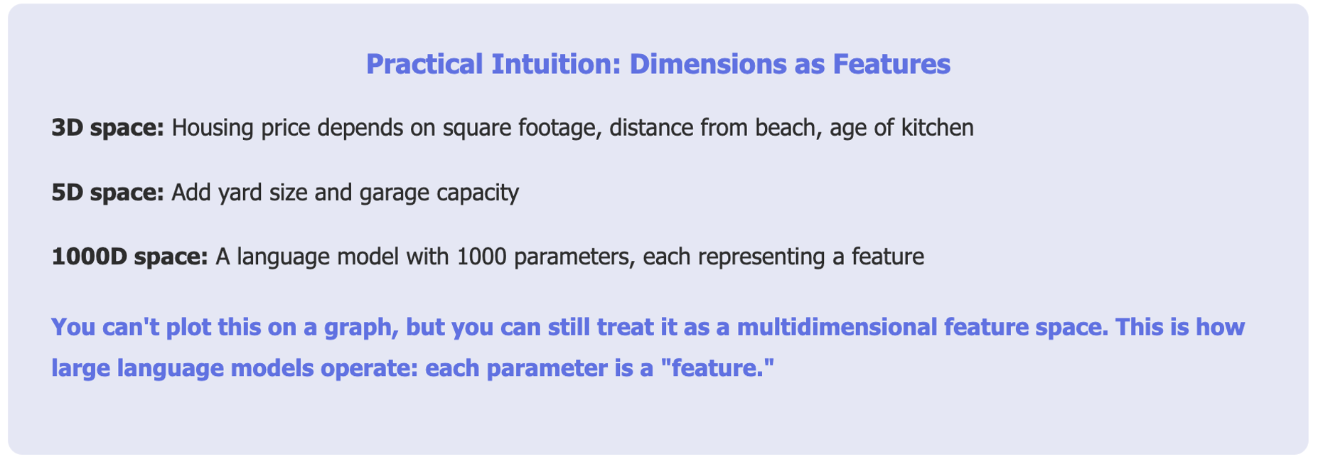
A more intuitive way is to think of dimensions as features.

Take housing prices:

3D space: price depends on square footage, distance from the beach, and the age of the kitchen.
5D space: now add yard size and garage capacity.

You can’t plot this on a normal graph, but you can still treat it as a 5-dimensional feature space.

This is how large language models operate: each parameter is a “feature.”

For example, if your model has parameters representing a German female, you’ll likely find a German male nearby, offset by a certain “gender vector.” If you take that same offset and apply it to French female, you’ll land near French male.

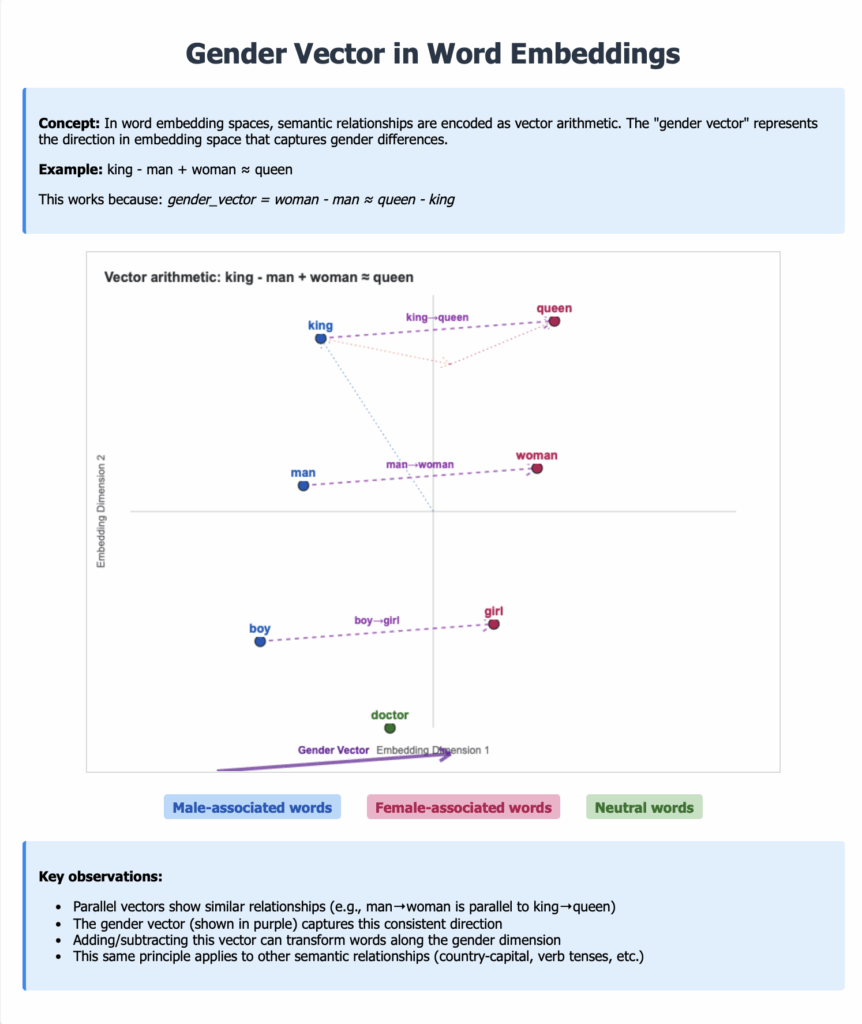
The diagram shows gender vectors in word embeddings. The concept is that in word embedding spaces, semantic relationships are encoded as vector arithmetic. The “gender vector” represents the direction in embedding space that captures gender differences.

For example, king is to man as woman is to queen.

This works because there is a gender_vector. The vector expresses the mathematical concept of gender. When the gender vector is applied to a ‘male’ word it shifts ‘boy’ or ‘man’ or ‘king’ in one direction. And likewise, it shifts ‘girl’ or ‘woman’ or ‘queen’ in a different direction.

The key observations of gender vectors:

Parallel vectors show similar relationships (e.g., man→woman is parallel to king→queen)

The gender vector (shown in purple) captures this consistent direction

Adding/subtracting this vector can transform words along the gender dimension

This same principle applies to other semantic relationships (country-capital, verb tenses, etc.)

That offset is a vector transposition in a high-dimensional space.

Key Takeaways

Summary: Matrix Transformations in Machine Learning:

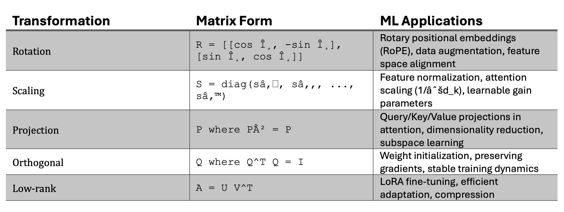
Essential Formulas to Remember

Linear transformation:y = Ax (matrix-vector product applies the transform)
Composition:(AB)x = A(Bx) (multiply matrices to combine transforms)
Vector arithmetic in embeddings:king is to man as queen is to woman.
Semantic relationships encoded as consistent vector directions.

Foundational Papers:

Attention & Transformers: “Attention Is All You Need” (Vaswani et al., 2017) – Original transformer architecture
Word Embeddings: “Efficient Estimation of Word Representations in Vector Space” (Mikolov et al., 2013) – Word2Vec introduction
Low-Rank Adaptation: “LoRA: Low-Rank Adaptation of Large Language Models” (Hu et al., 2021)
Rotary Embeddings: “RoFormer: Enhanced Transformer with Rotary Position Embedding” (Su et al., 2021)

Textbooks & Courses:

Linear Algebra: “Introduction to Linear Algebra” by Gilbert Strang (MIT OpenCourseWare available)
Deep Learning: “Deep Learning” by Goodfellow, Bengio, and Courville (free online)
NLP with Transformers: “Natural Language Processing with Transformers” by Tunstall, von Werra, and Wolf

Interactive Resources:

The Illustrated Transformer – Visual guide to attention mechanisms
TensorFlow Embedding Projector – Explore word embeddings interactively
How to Use t-SNE Effectively – Understanding embedding visualizations

In the next article, we’ll explore projection and how it lets us focus on the most important dimensions of complex data.

Date

December 6, 2025

Tags:

Math