Math for Deep Learning III – Linear Layer Collapse

Contents

Introduction

Linear Datasets

Non-linear Datasets

Why It Can’t Collapse

This is Why LLMs Work

The Mathematical Barrier

Measuring Linear Collapse

Measuring Linear Collapse

Final Notes

Introduction

Previously we learned how to transform one matrix with another. We learned that the fundamental property of LLMs is learning through this process: Training uses matrix transformation to adjust weights.

This article is an aside to strengthen your main AI building muscles by learning some of the weaknesses that had to be overcome during their development. Think of this article as a training exercise to build accessory muscles that you need for full body strength.

Like those exercises, this article will be short and light weight. You can read it repeatedly until you master the contents!

Linear Datasets

Imagine that we are trying to learn the border between two groups of dots, red and blue. If the two groups are each opposite sides of the border, then we call this a linear dataset, because we can draw a line between the two groups and define them:

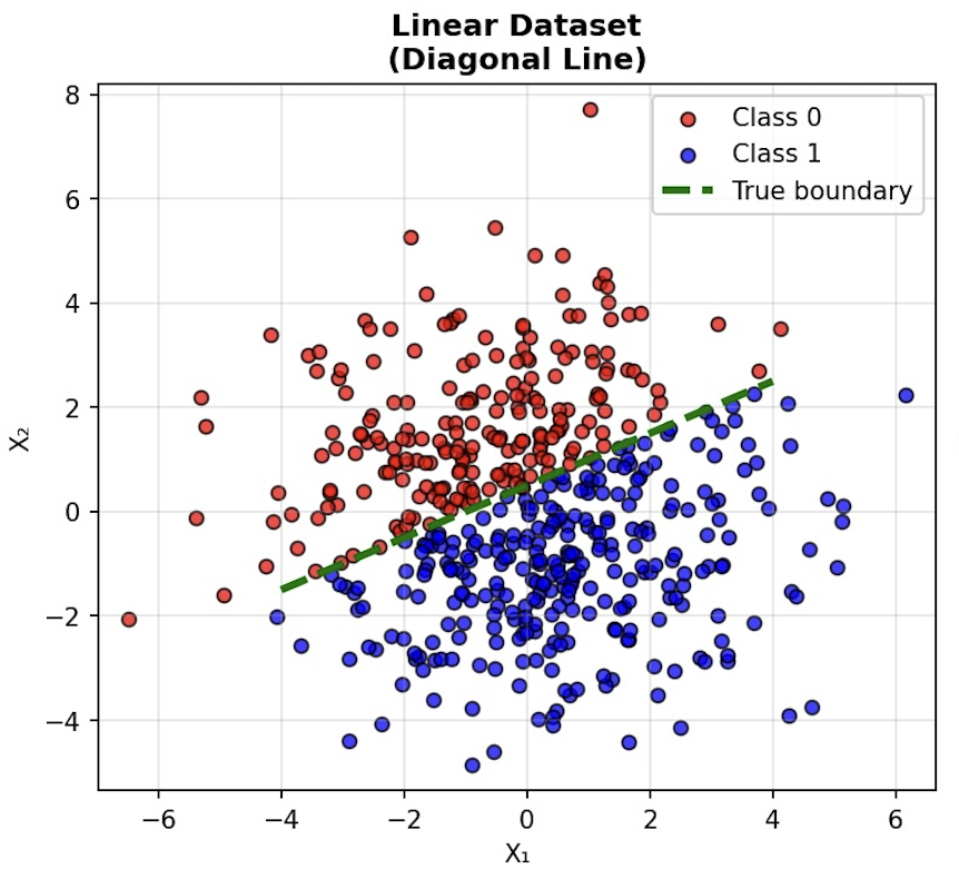
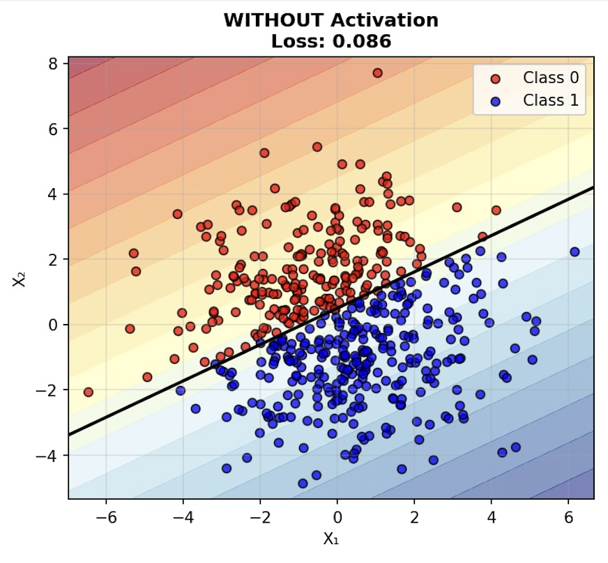
If we train a network on the positions of dots on either side of a linear boundary, the network will learn that boundary. This works even without activation functions because we only need a straight line to define a linear dataset—and a network without activation functions can represent any straight line (or hyperplane in higher dimensions).

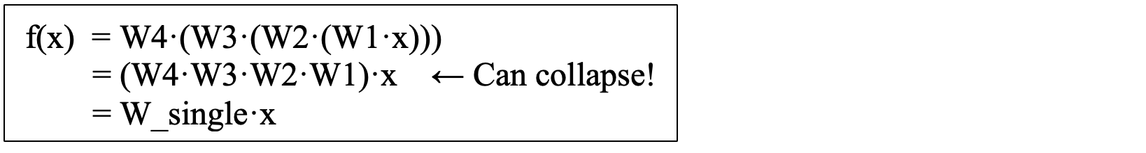
If we think about what is happening in this type of training, we are multiplying a matrix of positions in the input matrix ‘x’ times a weight matrix. We can call the weight matrix ‘W1’ for layer 1; ‘W2’ for layer 2; ‘W3’ for layer 3 and so on. As we train these multiple layers, the result can be thought of as:

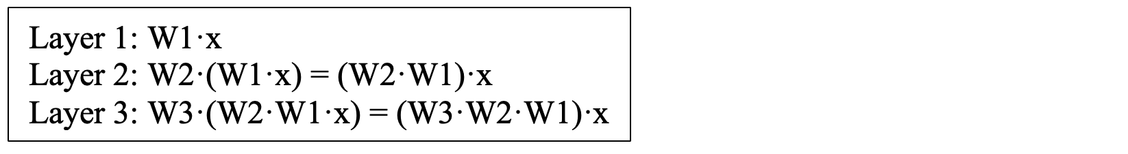
And you can see that for each layer, we always have a linear equation, in the form of our standard linear equation, y = mx + b. (However in this example m is a matrix called ‘W’ and b is an array of values each set to zero.)

No matter how many layers you stack, without an activation function, it’s mathematically equivalent to a single linear transformation. The layers “collapse” into one matrix multiplication.

The problem with this is that you can’t learn complex, nonlinear patterns.
The solution is to add activation functions between layers.

Non-linear Datasets

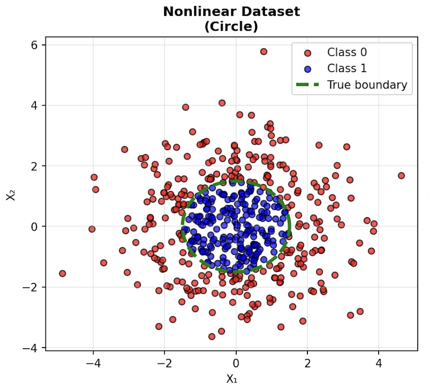
Now imaging that we have a non-linear dataset. We can informally define this as a dataset we can’t subdivide with a straight line. The figure shows a non-linear dataset as a cluster of blue dots inside a larger cluster with the outer dots colored red. In code, we create this dataset starting with a random cluster of dots, and those within 1.5 units from the origin are colored blue, the rest are colored red:

This is where the network without activation ‘collapses.’ The term of art is ‘collapse’ but what we are really expressing is a limitation of networks without an activation function. In this case, we see the network really failing to find any boundary between the red and blue dots. Instead, as you can see from the position of the black line in the image below, it appears to find a boundary between the areas with dots and the area with no dots at all. As before, if we simply train our network without an activation function, it will collapse:

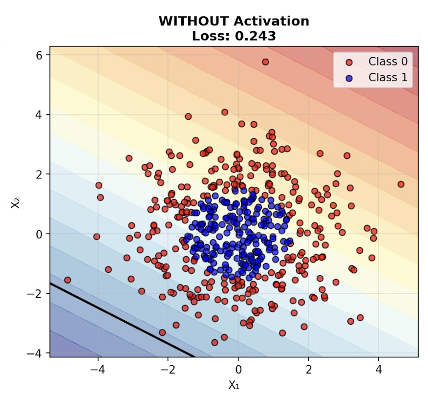
Without Activation (Collapsible):

However, if we train our network with an activation function (which we designate as σ), then it will not collapse and it can recognize our circle of blue dots:

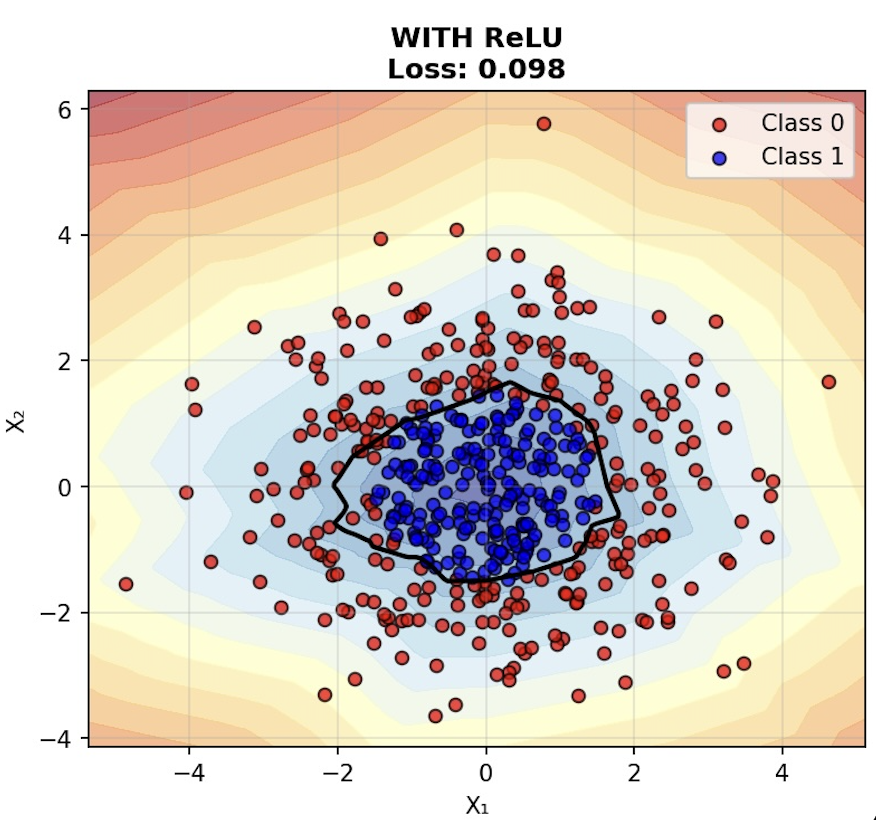
With Activation (NOT Collapsible):

Where σ is the activation function (like ReLU or sigmoid).

Why It Can’t Collapse

Let’s expand it step by step:

You cannot pull the σ functions out or combine them with the weight matrices because:

• σ is nonlinear (ReLU, sigmoid, etc.).
• Matrix multiplication is linear
• Any composition of linear + nonlinear cannot be replicated by any single linear transformation.

This is Why LLMs Work

Well, it’s not the only reason. But this rather simple and seemingly mundane fact – that networks of equations containing relu functions or sigma functions cannot collapse – is the underpinning of why large language models with billions of parameters and hundreds of layers succeeds at all.

Because of the non-linear transformation of the sigma function.

This non-linear transformation means that the values of one layer are NOT simply multiples of values in another layer.

If they were, then the values in any single layer would be a trivial multiple of the values in some other layer. And as such, they would not add new information to the network.

You might ask, if this is  barrier, how does the brain itself overcome this? Isn’t the brain trained by linear input of signals at synapses? The answer is that for simple signals, like those that carry a pain signal from your fingertip to your brain, a simple signal across a single synapse might be the primary event. But in your brain, during training, neurons do not have one input. They have multiple inputs. And the processing of multiple inputs to an output signal is the biological equivalent of the sigma function. It’s the non-linear event where the magic happens.

We can call this The Mathematical Barrier. This barrier prevents any single layer from merely representing a mathematical multiple of some other layer.

The Mathematical Barrier

Without activation: Linear ∘ Linear ∘ Linear = Linear ✓ (can collapse)

With activation: Linear ∘ Nonlinear ∘ Linear ∘ Nonlinear ≠ Linear ✗ (cannot collapse)

This is exactly what makes deep learning powerful—each activation function creates a “barrier” that prevents the layers from collapsing into one!

The following image shows how networks can distinguish between linear or non-linear datasets and is available here.

Measuring Linear Collapse

We talked about linear and non linear datasets in the context of training with and without a sigmoid function. Some nonlinear function must be part of the training. But let’s go back to look more deeply. Is a linear collapse something that we can measure? And what I mean is: can we quantify the types and severities of failures of different types of training?

Yes, linear collapse is absolutely measurable, and there are several concrete metrics we can use to both detect it and quantify failure severity. Let me walk through the key approaches.

Types of Collapse

1. Effective Rank of the Composed Transformation

When you stack linear layers without activation functions, the entire network collapses to a single matrix multiplication: W_total = W_n · W_{n-1} · … · W_1. This is something we talked about above. You can measure the effective rank of this composed matrix using singular value decomposition. A “collapsed” network will have effective rank ≤ min(input_dim, output_dim), regardless of how many parameters you have. Typically a failed training where there are no nonlinear sigmoid contributors will have a rank close to 2-3. This is how you know it failed.

2. Representational Similarity Analysis

You can compute correlation or centered kernel alignment (CKA) between layer activations. In a healthy deep network, representations should progressively transform. In linear collapse, layer representations become nearly identical linear projections of each other. This is not really that different from effective rank: You are measuring the similarity between layers and noticing that they are linear multiples of one another.

3. Decision Boundary Complexity

We can also use probe datasets with known non-linear structure (XOR, spirals, concentric circles). A collapsed network literally cannot solve these—not because of poor training, but because the solution space doesn’t contain the answer.

You can visualize this collapse in my interactive demo by downloading the github python gist and running it locally. The following screenshot shows how it can utilize a tanh nonlinear function to actually learn the pattern of blue and red dots in a spiral. When using the tanh function as in the screen shot, you can see the network is NOT collapsed. The place to look is at the spiral and the background. As the model ‘learns’ the spiral, it fills in the background with the correct color. You can see in the screenshot that the model is learning the red arm of the spiral and has begun to learn the blue arm as well. It’s making goor progress by the 689^th epoch of training.

You can run the same simulation with the ‘none’ setting to simulate the lack of a non-linear sigmoid function. This setting will never reach a point where it approximates the shape of the spiral. In that case, look for how the blue and red backgrounds never get near approximating a spiral shape.

Demo Linear Collapse With Numbers

If you are like me, you like to see ALL the numbers as they change during a collapse. I have another demo for this. In this demo, you can see the numbers of each network component change as the network learns the input values. Again, you can select to either use no activation or to use a sigmoid activation. But here you can see

Final Notes

This is not the ONLY  reason why LLMs work. But the fact that sigmoid functions introduce a non-linear quality to training is critical. This demonstrates the prime importance of the activation function.